2.1 Model

To investigate the oceanic sensitivity of the GrIS throughout the last two glacial cycles, we use the three-dimensional, hybrid, ice-sheet–shelf model GRISLI-UCM. The model is an extension of the GRISLI ice-sheet model (Ritz et al., 2001), which has already been successfully used to simulate the evolution of the past Greenland (Quiquet et al., 2012, 2013) and Antarctic ice sheets (Ritz et al., 2001; Philippon et al., 2006; Alvarez-Solas et al., 2010), as well as the Laurentide Ice Sheet (Alvarez-Solas et al., 2011, 2013). GRISLI-UCM combines the Shallow Ice Approximation (SIA) for slow inland deformational flow and the Shallow Shelf Approximation (SSA) over fast-flowing areas, that is, ice streams and ice shelves, where plug flow is dominant. Since we assume deformational ice-sheet regions to be frozen at the bedrock, no basal sliding is considered for SIA-dominated areas. Basal sliding for ice streams is determined through a basal drag term (τ_b), defined as a function of the effective pressure (N_eff) between ice and water pressure, and the basal horizontal velocity (u_b), considered as follows:

where

Dragging at the floating ice-shelf base is considered to be zero. The position of the grounding line is evaluated following a flotation rule dependent on the current sea level and the ice thickness. Calving at the ice front is based on a two-condition thickness criterion (Peyaud et al., 2007; Colleoni et al., 2014). First, an ice-shelf front must have a thickness lower than 200 m to potentially contribute to ice discharge. This threshold is in agreement with the thickness of many observed shelves at their ice–ocean interface. Second, if the ice advected from each upstream point is not sufficient to maintain the ice-front thickness higher than that threshold, the grid point at the front calves. The entire GrIS ice dynamics is solved on a computational grid of 20 km × 20 km horizontal resolution and 21 vertical layers. The glacial isostatic adjustment (GIA) is described by the elastic lithosphere – relaxed asthenosphere method (Le Meur and Huybrechts, 1996), for which the viscous asthenosphere responds to the ice load with a tunable characteristic relaxation time (see Sect. 2.4).

The hybrid scheme uses a weighting function to combine the non-sliding horizontal SIA velocities (u_SIA) with the SSA horizontal velocities (u_SSA) and is defined as (Bueler and Brown, 2009)

where the weighting function f(u_SSA) depends on the module of the SSA component (u_SSA) through

ranging between 0 and 1. In this work, the reference velocity u_ref is set to 100 m a⁻¹. For small values of u_SSA, f(u_SSA)≈0 and the horizontal velocities are calculated within the SIA, while f(u_SSA)≈1 for u_SSA≫u_ref, for which the contribution of SSA dominates.

2.2 Atmospheric forcing

The surface mass balance (SMB) is calculated by the positive degree-day (PDD) scheme (Reeh, 1989) forced by surface atmospheric temperatures and precipitation. This melting scheme is admittedly too simple for palaeo-simulations as it omits the contribution of insolation-induced effects on surface melting, which are important in past warmer periods such as the Eemian (Robinson and Goelzer, 2014). However, since this study focuses on the melting effects induced by past ocean temperature variations, the PDD melt model is sufficient to give a first approximation of surface melt that allows the ice sheet to retreat during interglacial periods in a realistic way. The atmospheric temperature forcing is a spatially and temporally variable field. It is retrieved using an index-anomaly approach in which the present-day climatological field (T_{clim, atm}) is perturbed by past temperature anomalies derived through a spatially uniform climatic index α(t) (Fig. 1), as follows:

The index α(t) is built through a multiproxy approach. First, we combine the temperature reconstruction for Greenland by Vinther et al. (2009) from 11.7 ka BP to present, the North Greenland Ice Core Project (NGRIP) reconstruction (Kindler et al., 2014) for 115–11.7 ka BP and the North Greenland Eemian Ice Drilling (NEEM) reconstruction (NEEM, 2013) for 135–115 ka BP, and we generate a synthetic temperature anomaly time series for 250–135 ka BP based on Antarctic isotope records following Barker et al. (2011). Second, the composite signal undergoes a windowed low-pass frequency filter ($f_{\text{c}}=\mathrm{1}/\mathrm{16}$ ka⁻¹) in order to remove the spectral components associated with millennial timescales and below. Finally, the index α is obtained by normalizing the resulting signal to be in agreement with Eq. (5), i.e. α=0 for the LGM and α=1 for the present day. The present-day climatological field is taken from the regional climate model MAR forced by ERA-Interim (Fettweis et al., 2013). T_{LGM, atm}−T_{PD, atm} is the 2-D surface atmospheric temperature (SAT) difference between the LGM and the present, as simulated by the climatic model of intermediate complexity CLIMBER-3α (Montoya and Levermann, 2008). For the precipitation rate, the procedure is similar, but the annual present-day precipitation is scaled by the ratio of the past precipitation to its present value, as in Banderas et al. (2017). At the base of the grounded ice, the melt rate is calculated as a function of the geothermal heat flux, which is prescribed following Shapiro and Ritzwoller (2004), and the local pressure melting point. The submarine melt rate is described in detail in the next subsection.

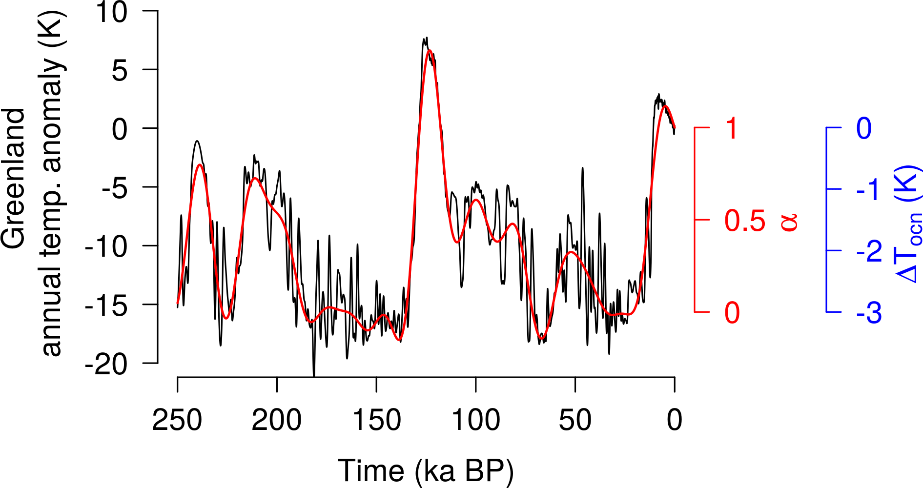
Figure 1The 250 ka Greenland annual temperature anomaly signal built through a multiproxy approach based on the reconstruction by Vinther et al. (2009) from 11.7 ka BP to present, the NGRIP reconstruction (Kindler et al., 2014) for 115–11.7 ka BP, the NEEM reconstruction (NEEM, 2013) for 135–115 ka BP and a synthetic temperature anomaly time series for 250–135 ka BP following Barker et al. (2011) (black line). The red line shows the filtered and normalized climatic index α used to correct the present-day climatological fields when forcing the model. The same signal can be interpreted as the palaeo-oceanic temperature anomaly of Eq. (8) (in blue).

Download

2.3 Oceanic forcing

Several marine basal melting rate parameterizations can be found in the literature. Generally, the submarine melt rate is thought to be directly influenced by the oceanic temperature variations below the ice shelves. Accordingly, most basal melting parameterizations are built as function of the difference between the oceanic temperature at the ice–ocean boundary layer and the temperature at the ice-shelf base, generally assumed to be at the freezing point. The dependence on this temperature difference can be linear (Beckmann and Goosse, 2003) or quadratic (Holland et al., 2008b; Pollard and DeConto, 2012; DeConto and Pollard, 2016; Pattyn, 2017). Because of the increasing temperature anomaly approaching the onshore ice-shelf limit, both schemes ensure a higher basal melting rate close to the grounding line, as suggested by observations (Dutrieux et al., 2013; Rignot and Jacobs, 2002; Wilson et al., 2017).

The marine basal melting rate parameterization used in this work follows a linear approach that accounts separately for sub-ice-shelf areas near the grounding line and for purely floating ice (ice shelves). A linear scheme is the simplest case that allows testing of the GrIS sensitivity to past oceanic temperature changes. The formulation is derived from the net basal melt rate B_gl (m a⁻¹) for ice-shelf cavities close to the grounding line and terminating in shallow ocean zones, expressed by Beckmann and Goosse (2003) as

where T_ocn is the oceanic temperature close to the grounding line (K), T_f is the temperature at the ice base, assumed to be at the freezing point (K), and κ is the heat flux exchanged between ocean water and ice at the ice–ocean interface ($\mathrm{m}{\mathrm{a}}^{-\mathrm{1}}{\mathrm{K}}^{-\mathrm{1}}$). Since knowledge of past T_ocn and T_f is challenging for the complex heat-flux transfer between ice shelves and the surrounding water, we opted for substituting these quantities and rearranging the equations to make them more suitable for palaeo-studies. A representation of the transient oceanic temperature T_ocn can be given by the climatological oceanic temperature T_{clim, ocn} corrected by the LGM–present temperature anomaly (T_{LGM, ocn}−T_{PD, ocn}) scaled by the same climatic index α=α(t) used to correct the atmospheric climatological fields (Fig. 1). Under this assumption, Eq. (6) can be rewritten as

where

Combining and reorganizing these equations as

we can finally retrieve the expression for the basal melting rate at the grounding line B_gl (m a⁻¹) as used in this work:

B_ref (m a⁻¹) $=\mathit{\kappa }(T_{\text{clim, ocn}}-T_{\text{f}})$ is assumed to represent the present-day basal melting rate around the ice sheet, κ represents the sensitivity of the basal melting rate to changes in the oceanic temperature, and ΔT_ocn (K) expresses the temporal evolution of the melting at the ice base. In this way, B_gl coincides with the present-day melt (B_ref) for α=1 and its LGM (21 ka BP) value for α=0. When B_gl is negative, the model allows for refreezing, and the grounding line can advance offshore.

In a more realistic setup, all parameters in Eq. (10) could be described by 2-D spatially variable fields. However, for the sake of simplicity, here we considered all the parameters to be spatially uniform around all the GrIS marine borders, as described in Sect. 2.4. The glacial–interglacial temperature anomaly T_{LGM, ocn}−T_{PD, ocn} (Eq. 8) is set constant to −3 K, which corresponds to the mean value of the reconstructed LGM sea surface temperature (SST) anomalies for the Atlantic Ocean between 60 and 80^∘ N latitude (MARGO Project Members, 2009). This value slightly differs from the LGM mean SST anomaly reconstructed by Annan and Hargreaves (2013) (between −1 and −2 K). However, a variation in κ or an identical change in ΔT_ocn equally affect the oceanic forcing applied to the model. Therefore, considering a different value for ΔT_ocn would not alter the magnitude of the oceanic sensitivity applied to the GrIS. These simplifications allow here for a spatially uniform, but time-dependent, B_gl.

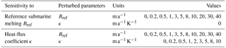
Table 1Summary of all parameter values used to perturb the basal melting rate equation (Eq. 10) in each sensitivity test.

Download Print Version | Download XLSX

The basal melting rate for purely floating ice shelves (B_sh) is given by the grounding-line basal melt B_gl scaled by a constant factor γ:

In this study, γ is set to 0.1. Hence, we consider that the basal melting rate for ice shelves is 10 times lower than that close to the grounding zone, which is qualitatively in agreement with melt rates observed in some Greenland glaciers (Münchow et al., 2014; Rignot and Steffen, 2008; Wilson et al., 2017). Conversely, the melt rate in the open ocean, that is considered as being beyond the continental shelf break, is prescribed to a high value (50 m a⁻¹) to avoid unrealistic ice growth beyond 1500 m of ocean depth.

2.4 Experimental design

To study how oceanic changes impact the evolution of the GrIS over the last glacial cycles, we performed a set of sensitivity tests by perturbing the two key parameters of the basal melting rate equation (Eq. 10): the estimated present-day submarine melting B_ref and the heat-flux coefficient κ. For each experiment, we ran an ensemble of simulations over the GrIS domain throughout the last 250 ka. In this study, the model is initialised with the present-day Greenland topography (Bamber et al., 2013), the characteristic relaxation time for the lithosphere is set to 3000 years, and the model is forced by the past relative sea-level reconstruction of Grant et al. (2014). The first ∼ 100 ka of the simulation are considered as a spin-up and are not analysed. A summary of all the parameter values used in each sensitivity test is shown in Table 1.

First, we analyse the sensitivity of the model to different constant (in space and time) B_ref values applied at the base of the ice-sheet marine margins. Due to the scarcity of submarine melt observations along the GrIS coasts, and since the only available estimates have focused on few very rapid tidewater Greenland glaciers that cannot be representative of the basal melt rate for the entirety of GrIS marine areas (Rignot et al., 2010; Motyka et al., 2011; Straneo et al., 2012; Xu et al., 2013; Enderlin and Howat, 2013; Fried et al., 2015; Rignot et al., 2016; Wilson et al., 2017), we assume present-day basal melting rates for Greenland comparable to those from Antarctic ice shelves (Rignot et al., 2013). The range of values of B_ref is set between 0 and 40 m a⁻¹, while κ is set to zero to make the ocean contribution constant in time. The resulting basal melting rate is thus equal to the tested B_ref value and a condition of no oceanic basal melting around the GrIS is achieved only when both B_ref and κ are set to zero.

Second, we study the sensitivity of the GrIS to the basal melt rate sensitivity κ at the ice–ocean interface. The range of tested values for κ is between 0 (expressing a temporally constant basal melting rate) and 10 $\mathrm{m}{\mathrm{a}}^{-\mathrm{1}}{\mathrm{K}}^{-\mathrm{1}}$. The choice of this range reflects the inference made in Antarctica by Rignot and Jacobs (2002) that a variation of 1 K in the effective oceanic temperature changes the melt rate by 10 m a⁻¹ (Eq. 6). Due to the lack of data for Greenland, as a first approximation, we can assume such a value is also realistic there. This is surely a simplification of the problem, as the relation between ocean temperature and melt rate is not universal but depends on many factors, such as the water salinity, the depth, the conformation of the cavity, the water velocity below the ice shelf and subglacial discharge. The sensitivity test for κ is firstly done for B_ref=1 m a⁻¹ and then for other B_ref values to show that the GrIS response to the melting rate sensitivity κ depends on the chosen reference basal melting rate (see Table 1).

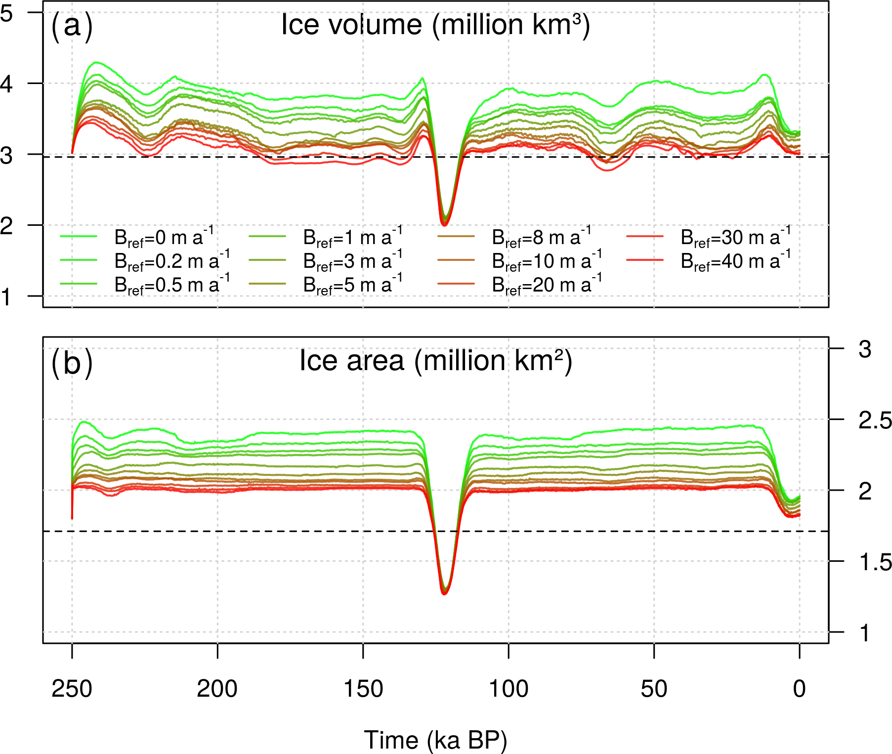
Figure 2Time evolution of (a) grounded ice volume (million km³) and (b) ice-covered area (million km²) simulated for different values of B_ref (m a⁻¹) having set κ=0 (see Table 1). Dashed lines show the present-day estimated volume and area of the GrIS (Bamber et al., 2013).

Download

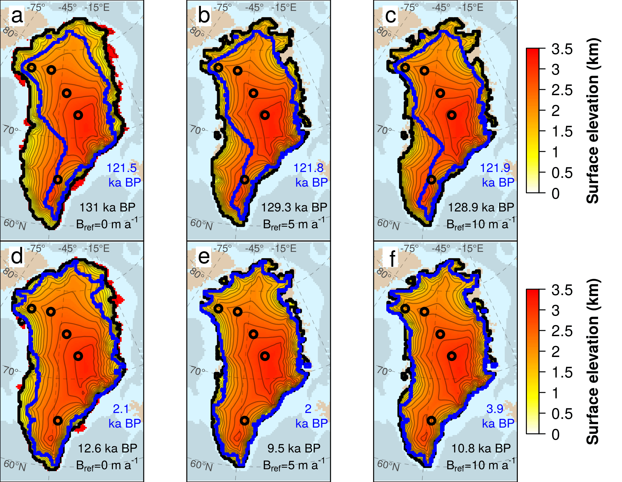
Figure 3Glacial maximum GrIS surface elevation (km) simulated at Termination II (a–c) and Termination I (d–f) for different values of the reference basal melting rate (B_ref=0, 5, 10 m a⁻¹) under constant oceanic conditions (κ=0). The timing at which the ice volume reaches its maximum value during a glacial cycle depends on the experiment and is stated in black for each snapshot. Blue lines indicate the GrIS extension at the following peak of deglaciation with its corresponding timing reported in blue. Red zones represent the ice shelves extending beyond the glacial maximum grounding line (black line). Black circles indicate the locations of the Camp Century, NEEM, NGRIP, GRIP and Dye3 ice cores (from north to south).

Download

3.1 Sensitivity to the reference submarine melting

In this experiment, the maximum ice volume reached in glacial times ranges between 3.4 and 4.3 million km³ (Fig. 2), 15–45 % higher than the observed current value (Bamber et al., 2013), suggesting that under constant oceanic forcing, the GrIS is limited to a configuration close to that of the present day (Fig. 3). The highest glacial ice volume is reached by imposing a null basal melting to the GrIS margins (B_ref=0), which corresponds to a simulation forced solely by palaeo-atmospheric variations. The varying SMB throughout the cycles still results in a changing GrIS ice volume over time. However, during glacials, most grounded ice remains on land above sea level, and only small ice shelves are able to grow (Fig. 3a, d).

For B_ref>0, a positive basal melt rate is applied to the marine margins of the whole GrIS throughout the two glacial cycles. The submarine melting not only inhibits the grounding-line advance during the glacials but contributes to thinning the few marine-terminating glaciers still present, constraining the grounding line further inland and resulting in a GrIS extent close to the observed present-day configuration (Fig. 3b, c, e, f). This mechanism can still be quite active during glacial times, such that the ice volume can be even lower than that simulated at the present (Fig. 2). Note that the ice volume is more sensitive to B_ref during the glacial periods, as during the interglacial periods the effect of the ocean is limited by the topography of the Greenland itself. Thus, the retreat is almost entirely driven by the surface ablation and the elevation–melt feedback. For low B_ref values, the ice lost in a deglaciation is to a large extent determined by the GrIS configuration in the preceding glacial. As high basal melting rates inhibit the ice growth during the cold phase, the higher the B_ref is applied to the marine margins, the lower ice loss is simulated in the following interglacial (Fig. 4). However, for B_ref=5 m a⁻¹, ice loss becomes insensitive to the melting applied, since the GrIS is also totally land based during glacial periods and any subsequent ice mass loss is therefore uniquely driven by ablation (compare Fig. 3a and b or Fig. 3d and e).

Figure 4Distribution of the ice volume (a) and area (b) lost during the LIG (triangles) and the Holocene (circles) as a function of B_ref. Grey and yellow shades show the range between the maximum glacial and the minimum interglacial ice volumes (area) for LIG and Holocene, respectively. The loss is calculated between the time at which the ice volume reaches its maximum value simulated before the deglaciation (between 132 and 128 ka BP for TII and between 13 and 9 ka BP for TI) and its following ice minimum (between 122 and 121 ka BP for the Eemian and between 8 and 0 ka BP for the Holocene). The colours of the points follow the legend of Fig. 2 for clarity. Each ice volume loss has been converted to value of sea-level-equivalent anomaly (m s.l.e. with respect to its simulated present-day volume.

Download

3.2 Sensitivity to the heat-flux coefficient

We next study the sensitivity to the ocean for a fixed B_ref value of 1 m a⁻¹ (Fig. 5). This value is within present-day submarine melting rates estimates, between those found in the largest remaining outlet glaciers in Greenland (Wilson et al., 2017) and those of smaller marine-terminating glaciers with presumably much lower ocean-induced melt. Under this assumption, the maximum ice volume simulated in both glacial periods for different κ values ranges between 4 and 5.4 million km³, greatly exceeding the range found for the case with constant oceanic forcing. Prescribing positive or zero uniform submarine melting to the marine boundaries limits the glacial expansion of the GrIS (Figs. 6a and 7a), as discussed in Sect. 3.1. Conversely, by intensifying the oceanic forcing applied to the margins (with increasing values of κ), the glacial ice volume increases. For κ=1 $\mathrm{m}{\mathrm{a}}^{-\mathrm{1}}{\mathrm{K}}^{-\mathrm{1}}$, the model simulates a GrIS glacial expansion to the continental shelf break in which the grounding line has already advanced from the present-day continental boundaries, and large ice shelves are generated in the eastern GrIS, especially in the northeast (Figs. 6b and 7b). The maximum expansion is simulated for the last glaciation, where the grounding line has almost reached the continental shelf break and large ice shelves in the east cover the remaining shallower zones of the bathymetry. For κ=10 $\mathrm{m}{\mathrm{a}}^{-\mathrm{1}}{\mathrm{K}}^{-\mathrm{1}}$, the GrIS extends all the way to the continental shelf break at its glacial maximum, while only a few small floating ice shelves are present (Figs. 6c and 7c).

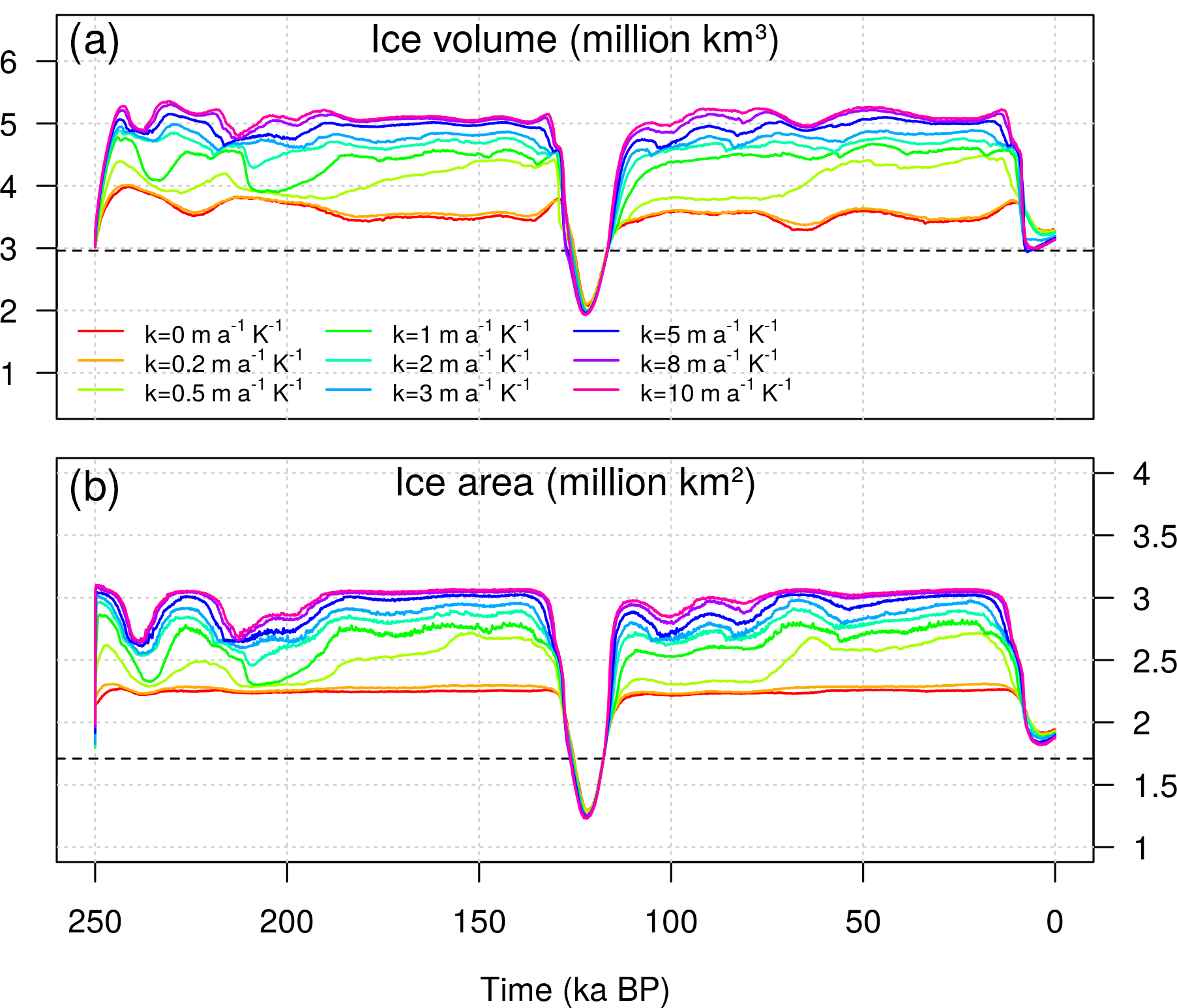
Figure 5(a) Time evolution of GrIS grounded ice volume (million km³) and (b) ice area (million km²) simulated for different values of the heat-flux coefficient κ, having set B_ref=1 m a⁻¹. Dashed lines shows the GrIS ice volume and area estimated for the present day (Bamber et al., 2013).

Download

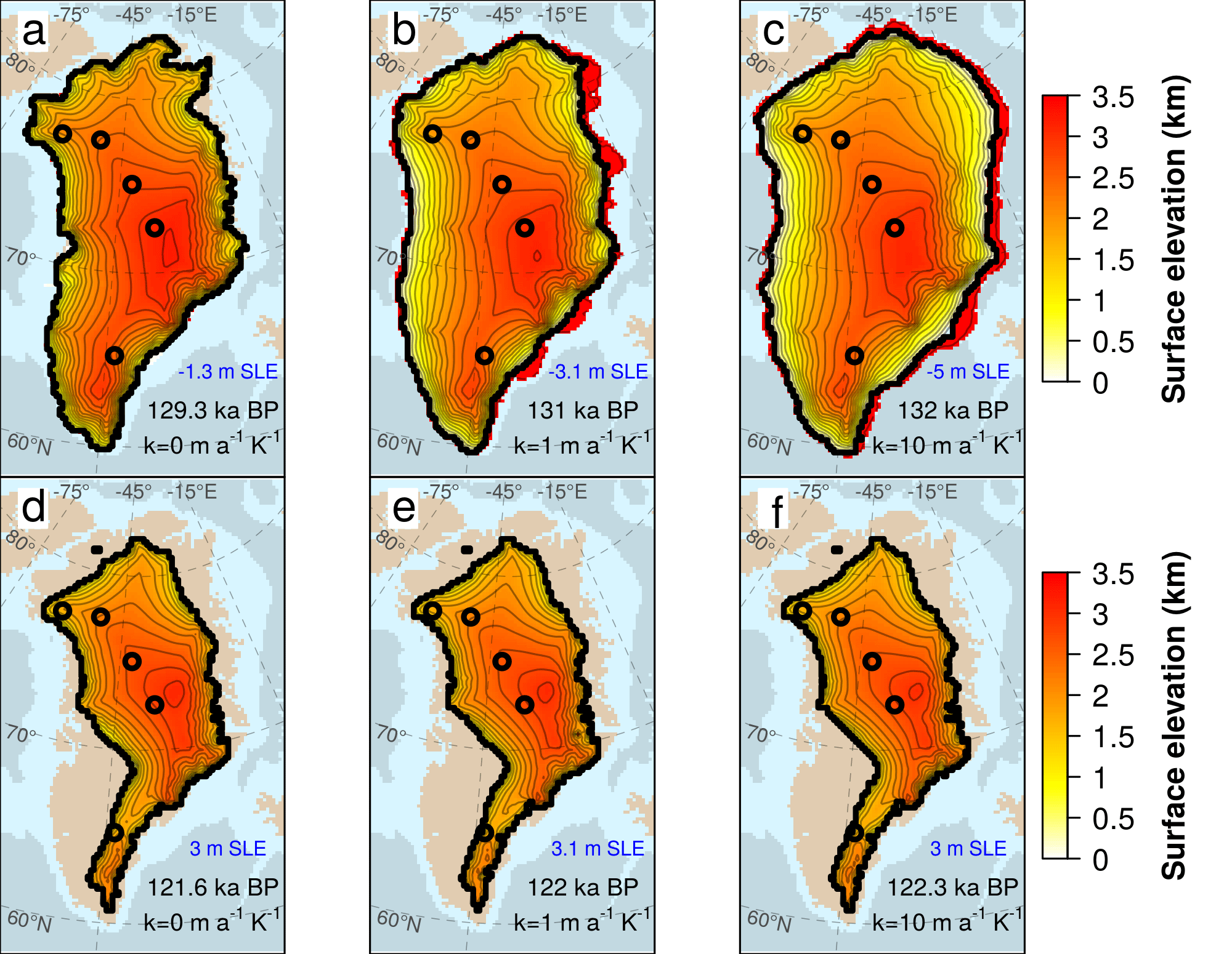
Figure 6GrIS surface elevation (km) simulated at the penultimate glacial maximum (TII) (a–c) and at the LIG minimum (Eemian) (d–f) for three values of the melting rate sensitivity κ having set B_ref=1 m a⁻¹. The timing of these snapshots depends on the experiment and is stated in black for each snapshot. Corresponding ice volume (in s.l.e.) is shown in blue. Red zones represent the ice shelves extending beyond the glacial maximum grounding line (black line). Black circles indicate the locations of the Camp Century, NEEM, NGRIP, GRIP and Dye3 ice cores (from north to south).

Download

Figure 7GrIS surface elevation (km) simulated at the LGM (TI) (a–c) and present-day GrIS (d–f) for three values of the heat-flux coefficient κ having set B_ref=1 m a⁻¹. The timing of the snapshots depends on the experiment and is stated in black for each snapshot. Corresponding ice volume (in s.l.e.) is shown in blue. Red zones represent the ice shelves extending beyond the LGM grounding line (black line). Black circles indicate the locations of the Camp Century, NEEM, NGRIP, GRIP and Dye3 ice cores (from north to south).

Download

A larger ice sheet loses more ice during a deglaciation, leading to an interglacial state that is almost independent of κ (Fig. 5). This response is related to the saturation of the oceanic forcing in warm peaks, when the GrIS is almost totally land-based and the ice loss is hence mostly due to the increase in atmospheric temperature and precipitation. Since glacial accretion affects the ice growth much more than basal melting during the retreat, the ice loss during a deglaciation monotonically increases with increasing κ (Fig. 8). Thus, for larger κ values, more ice grows during glacial periods and more ice is lost, and faster, during the subsequent deglaciation. Mass loss is mostly due to the large number of grounded-ice zones that are converted into ice-free areas during the deglaciation (Fig. 8b). The percentage of grounded points lost until the peak of an interglacial period saturates for κ above 3 $\mathrm{m}{\mathrm{a}}^{-\mathrm{1}}{\mathrm{K}}^{-\mathrm{1}}$ in correspondence with preceding glacial GrIS configurations which present a grounding-line expansion to the continental shelf break. The slightly increasing ice loss still observed for higher oceanic sensitivities is mostly related to the ice lost in the GrIS interiors due to the positive elevation–melt feedback.

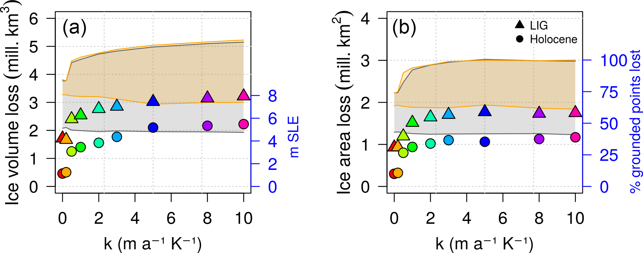
Figure 8Distribution of ice volume (a) and area (b) lost during the LIG and the Holocene as a function of κ, for B_ref=1 m a⁻¹. Grey and yellow shades show the deviation between the maximum and the minimum ice volumes (area) for LIG and Holocene, respectively (see Fig. 5). The loss is calculated between the time at which the ice volume reaches its maximum value simulated before deglaciation (between 140 and 128 ka BP for TII and between 19 and 10 ka BP for TI) and the subsequent ice minimum (between 122 and 121 ka BP for the Eemian and between 8 and 0 ka BP for the Holocene). The colours of the points follow the legend of Fig. 5 for clarity.

Download

Due to our melting parameterization (Eq. 10) and to the B_ref value chosen, water below the ice shelves is allowed to freeze for κ>0.5 $\mathrm{m}{\mathrm{a}}^{-\mathrm{1}}{\mathrm{K}}^{-\mathrm{1}}$, favouring ice growth and GrIS expansion (Fig. 5). Below this threshold, the model still allows for submarine melting rates across the margins in glacial times and the GrIS expansion is almost totally driven by surface accumulation. However, the sensitivity with respect to κ strictly depends on the value of B_ref, as it defines the positive threshold that the glacial GrIS has to overcome to start reacting to the oceanic forcing imposed at the margins (Fig. 9). For B_ref=10 m a⁻¹, the GrIS responds to the ocean only for κ>3 $\mathrm{m}{\mathrm{a}}^{-\mathrm{1}}{\mathrm{K}}^{-\mathrm{1}}$, while for B_ref=30 m a⁻¹ the GrIS starts to expand only for κ>8 $\mathrm{m}{\mathrm{a}}^{-\mathrm{1}}{\mathrm{K}}^{-\mathrm{1}}$. For high B_ref, since a constant high submarine melting is applied overall, the glacial GrIS is almost constrained to the PD configuration and exposure to the ocean is reduced. Only a sufficiently high κ to counteract this strong melting is able to make the GrIS expand and then retreat during the interglacial. Once the reaction has started, the sensitivity of the GrIS to κ increases with increasing B_ref; i.e. small variations in the magnitude of κ lead to a fast and large growth of ice during glacials and consequently to a fast and large loss of ice during the deglaciation. Similar results are found for the LIG (not shown).

3.3 Last interglacial

The amount of ice lost during the LIG period increases with the oceanic sensitivity κ. High κ values lead to higher glacial ice volumes and to larger ice losses during the consequent deglaciation (Fig. 8). The range of observed volume changes spans between 4.2 m s.l.e. (for κ=0) and 8 m s.l.e. (for κ=10 $\mathrm{m}{\mathrm{a}}^{-\mathrm{1}}{\mathrm{K}}^{-\mathrm{1}}$), above the present-day GrIS ice volume. Despite this large ice-loss range, all GrIS configurations simulated at the LIG ice minimum (Eemian) present a similar extension (Fig. 6d–f). In all experiments, a large retreat is observed in the north (especially in the northeast), where melting overcomes the low accumulation rates, and in the southwest, where the ice discharge from the interior is enhanced by the presence of fast ice streams and, in some areas, by the fact that the bedrock is below sea level. Although the position of the land-ice borders at the Eemian is not very sensitive to κ, the corresponding surface elevation fields show some differences depending on κ. For high values of κ, a lower ice elevation is simulated over the GrIS (compare Fig. 6d and f), a tendency that is reflected in a slightly lower ice volume too (Fig. 5).

It is interesting to note that even when imposing a very high κ, the complete disappearance of the GrIS is not simulated. The GrIS is only partly deglaciated and all ice-core sites are still covered by ice (including the discussed ice core locations of Dye3 and NEEM). Since the oceanic-driven retreat is limited by the land-based configuration observed in the interglacials, the retreat during the LIG is mainly controlled by the atmospheric temperatures and precipitations with which the model is forced.

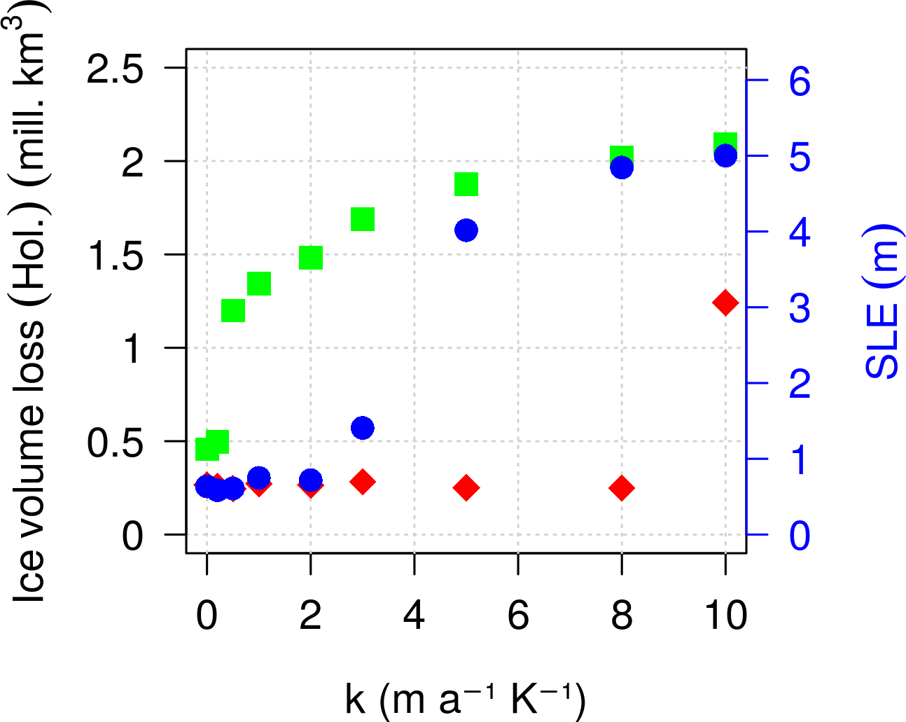
Figure 9Distribution of the ice volume lost in the Holocene as a function of the heat-flux coefficient κ, simulated for three selected reference basal melting rates (B_ref=1 m a⁻¹ in green, B_ref=10 m a⁻¹ in blue and B_ref=30 m a⁻¹ in red). The ice volume loss is calculated between the time at which the ice volume reaches its maximum value before the deglaciation and the present day. The green points are the same as the circles of Fig. 8a (for the Holocene).

Download

The amount of ice lost during the Eemian relative to the present day (Fig. 10), which ranges between 2.9 and 3.2 m s.l.e., is within the uncertainty range of ice volumes suggested by some previous studies (e.g. 1.2–3.5 m s.l.e. for Helsen et al. (2013), 0.4–4.4 m s.l.e. for Robinson et al. (2011) and 0.4–3.8 m s.l.e. for Stone et al., 2013). Also, the timing at which the peak of deglaciation occurs, which spans between 122.3 and 121.6 ka BP in all the simulations, agrees with the timing proposed in many previous studies (Calov et al., 2015; Langebroek and Nisancioglu, 2016; Robinson et al., 2011; Stone et al., 2013; Yau et al., 2016). The time at which the peak of the Eemian occurs in our experiments depends partly on the timing of the atmospheric temperature peak and partly on the duration of the post-glacial rebound, which controls the intrusion of warm waters into the GrIS bays enhancing the ocean-driven retreat. However, the Eemian peak does not depend on the maximum insolation since the PDD scheme used does not account for past insolation changes.

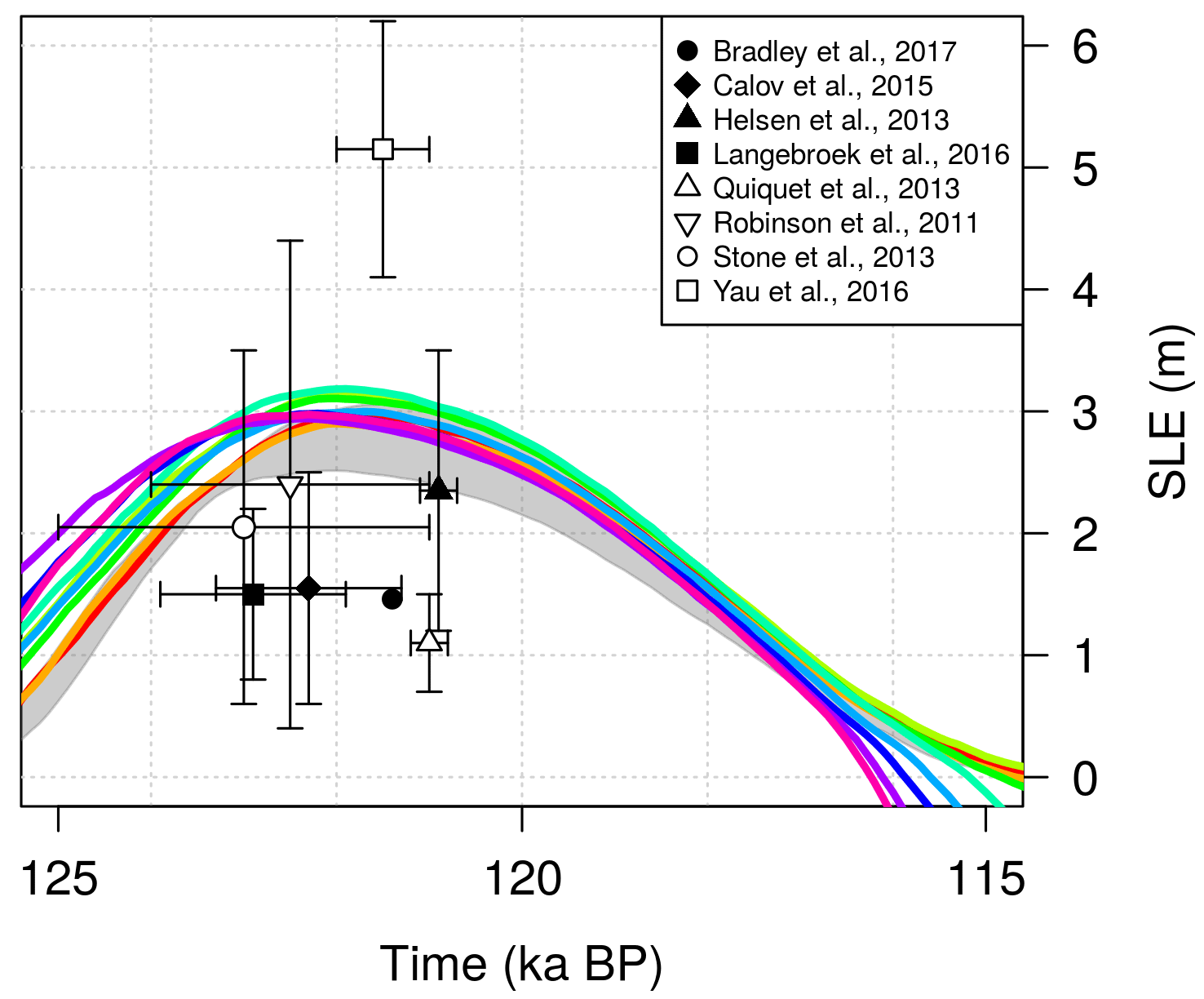
Figure 10GrIS ice volume evolution simulated for different values of the melting rate sensitivity κ during the last interglacial (see Fig. 5 for the line colour legend). The ice volumes have been converted to values of s.l.e. anomaly with respect to the present-day volumes estimated in each specific simulation. Grey shading represents the reference basal melting rates B_ref investigated for the case of constant-in-time oceanic forcing (κ=0 $\mathrm{m}{\mathrm{a}}^{-\mathrm{1}}{\mathrm{K}}^{-\mathrm{1}}$). The upper bound refers to B_ref=40 m a⁻¹ and the lower bound to B_ref=0 m a⁻¹. Black and white symbols indicate the LIG minimum ice volumes estimated by previous studies. The tight clustering of our estimates compared to previous work is due to the fact that the sole uncertainty is here related to the oceanic forcing through κ.

Download

3.4 Last Glacial Maximum

Although many uncertainties about the GrIS configuration during the last glacial period still exist, several estimates of the sea-level contribution from the GrIS during the last deglaciation can be found in the literature: 2.6 m s.l.e. (Bradley et al., 2017), 2.7 m s.l.e. (Huybrechts, 2002), between 2 and 3 m s.l.e. (Clark and Mix, 2002), 3.1 m s.l.e. (Fleming and Lambeck, 2004), 4.1 m s.l.e. (Simpson et al., 2009), between 3.1 and 4.5 m s.l.e. (Buizert et al., 2018) and 4.7 m s.l.e. (Lecavalier et al., 2014). These estimates come from ice-sheet models of different complexity, with their own dynamics and boundary conditions. Particularly the ice-sheet model used by Simpson et al. (2009) and Lecavalier et al. (2014) is run in combination with a GIA and RSL model and then constrained by past surface elevations derived from ice-core data, observations of past changes in RSL and the present-day GrIS configuration. These models do not solve the dynamics of the ice shelves or the grounding-line migration, which is parameterized. However, their estimates of the GrIS spatial extent can be considered as the most realistic reconstructions of the recent past glacial GrIS so far.

Under constant oceanic conditions, the LGM-PD ice excess simulated by our model at 21 kyr BP spans between 0 and 1.4 m s.l.e. for B_ref ranging from 0 to 40 m a⁻¹, increasing with decreasing B_ref values (grey shaded region – Fig. 11). This range is well below previous LGM ice volume reconstructions found in the literature (grey points). However, slightly larger ice volumes (0.6–2 m s.l.e.) are found at the peak simulated further in time in the glaciation (∼ 13–10 ka BP). For the case with no submarine melting (B_ref=0 m a⁻¹), the maximum ice volume (lower bound of grey shadow, at ∼ 12 kyr BP) is close to those of Huybrechts (2002) and Bradley et al. (2017). In this simulation, the GrIS increases moderately as its extension surpasses its PD borders and the grounding line approaches the continental shelf (Fig. 12a). Nevertheless, the atmospheric forcing alone is not sufficient to make the GrIS expand as expected during the LGM. According to reconstructions, the GrIS extended as far as the continental shelf break in every direction, except in the northeast region where the grounding line remains closer to the coast (Lecavalier et al., 2014). In our simulations, the GrIS reaches a glacial expansion consistent with the literature only for κ≥1 $\mathrm{m}{\mathrm{a}}^{-\mathrm{1}}{\mathrm{K}}^{-\mathrm{1}}$ (Fig. 12b). However, the ice volume reached for this oceanic sensitivity is still smaller than the LGM volumes of Simpson et al. (2009) and Lecavalier et al. (2014) (Fig. 11), since only with κ>3 $\mathrm{m}{\mathrm{a}}^{-\mathrm{1}}{\mathrm{K}}^{-\mathrm{1}}$ does the model simulate a maximum ice volume comparable to those ranges. The discrepancy in volumes, despite the same extension, could be related to the different dynamics and boundary conditions applied in the two models. Nevertheless, our simulated ice volumes are in agreement with recent estimates corrected for seasonal surface air temperatures in Greenland during the LGM (Buizert et al., 2018).

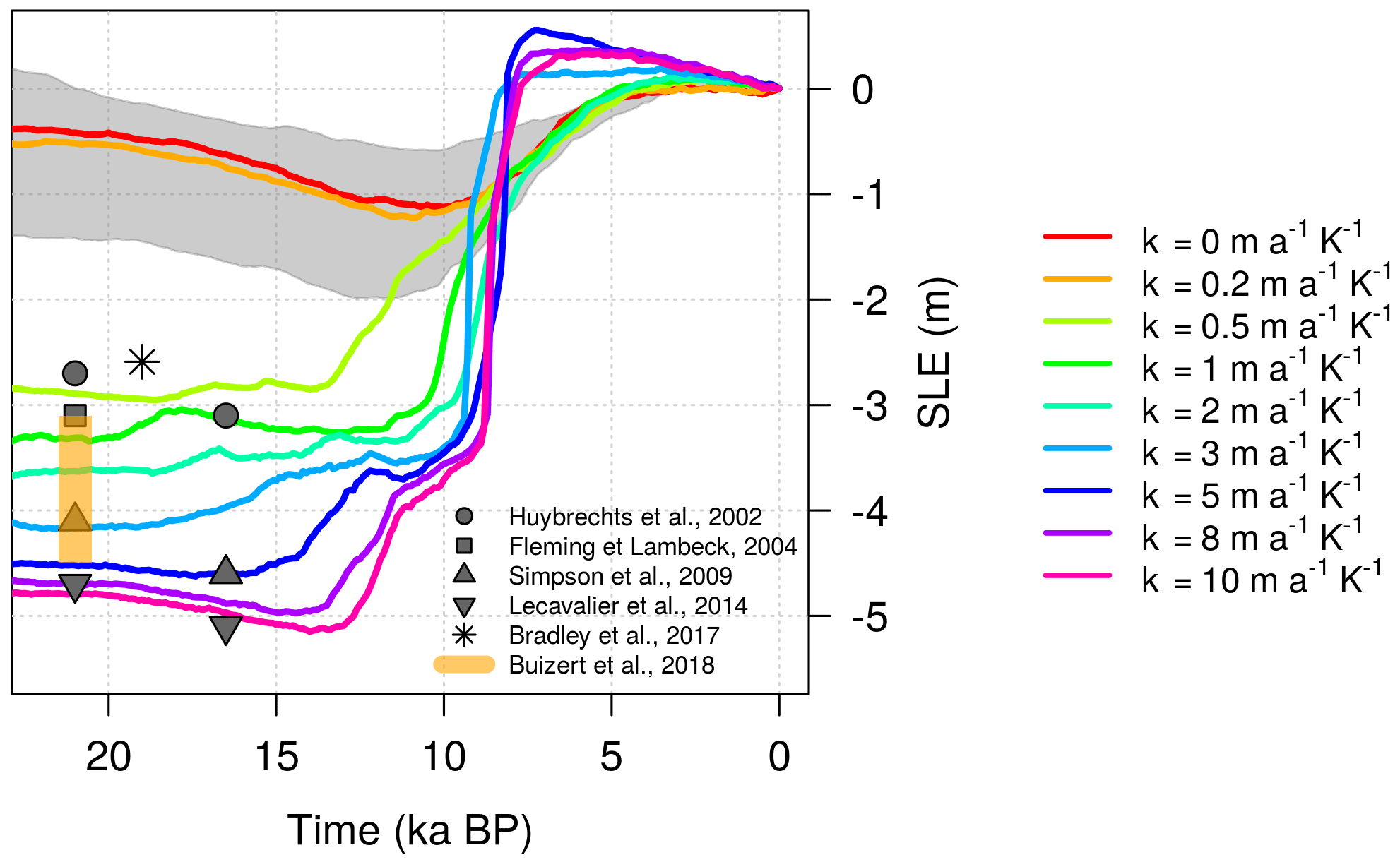
Figure 11GrIS ice volume evolution simulated for different values of the melting rate sensitivity κ during the last deglaciation. The ice volumes have been converted to values of s.l.e. anomaly with respect to the present-day volumes estimated in each specific simulation. As in Fig. 10, grey shading represents the simulations for the different reference basal melting rates (B_ref) investigated for the case of constant-in-time oceanic forcing (κ=0). The upper bound refers to B_ref=40 m a⁻¹ and the lower bound to B_ref=0 m a⁻¹. Grey dots and orange shading indicate estimates of the GrIS ice volume at the LGM (21 ka BP) and at the maximum ice volume reached before the last deglaciation (16.5 ka BP), as suggested by previous work.

Download

The timing of the reconstructed deglaciation can also provide information for comparison. The maximum increases suggested by Simpson et al. (2009) (4.6 m s.l.e.) and Lecavalier et al. (2014) (5.1 m s.l.e.) occur at 16.5 ka BP, while our simulations suggest a timing dependent on κ ranging from 20 to 10 ka BP for very low κ values (Fig. 11). The magnitudes of the oceanic sensitivity that best approximate the evolution of the GrIS before the Holocene are thus between 5 $\mathrm{m}{\mathrm{a}}^{-\mathrm{1}}{\mathrm{K}}^{-\mathrm{1}}$ (4.6 m s.l.e. at 17.4 ka BP) and 10 $\mathrm{m}{\mathrm{a}}^{-\mathrm{1}}{\mathrm{K}}^{-\mathrm{1}}$ (5.3 m s.l.e. at 14 ka BP). However, some discrepancies between our GrIS glacial extension and that of Lecavalier et al. (2014) are still present (Fig. 12b).

Figure 12GrIS total extent (ice shelves are included) simulated at the peak of the last glaciation for (a) no melting/freezing at the grounding line (cyan) and (b) κ=0, 1 and 10 $\mathrm{m}{\mathrm{a}}^{-\mathrm{1}}{\mathrm{K}}^{-\mathrm{1}}$ (red, green and purple lines, respectively) for B_ref=1 m a⁻¹. The timing of the glacial maximums is (a) 12 kyr BP and (b) 10, 20 and 14 kyr BP for κ=0, 1 and 10 m a⁻¹, respectively. LGM (21 kyr BP) GrIS grounding-line position estimated by Lecavalier et al. (2014) is shown for comparison (black line).

Download

3.5 Present-day GrIS

Given that the topography of the present-day GrIS is one of the trustworthy measures used to assess the reliability of an ice-sheet model, we compare our present-day GrIS ice thickness and extent simulated for κ=10 $\mathrm{m}{\mathrm{a}}^{-\mathrm{1}}{\mathrm{K}}^{-\mathrm{1}}$ to those estimated by Bamber et al. (2013) (Fig. 13). The choice of this particular κ value is based on the discussion above (Sect. 3.4) for the LGM and is supported by the good agreement between the simulated present-day ice volume and observations (Bamber et al., 2013) (Fig. 7f). The simulated extent of the GrIS matches reasonably well the observations. However, notable discrepancies are observed in some sectors. The main differences are found in the northeast, where GRISLI-UCM predicts an ice margin somewhat too far inland, and in the southwest, where our model is not able to make the GrIS retreat as expected. The ice loss in the north is a known problem that appears in many studies when simulating the GrIS during an interglacial (Stone et al., 2010; Born and Nisancioglu, 2012). In the interior, the difference in ice thickness is relatively low. However, the GrIS simulated by our model generally shows thicker ice along the margins, a tendency that propagates inland. Other areas in which our simulated ice thickness is lower than that observed are located in the centre of the continent and in the very southeast corresponding to a mountainous region. However, the focus of our work is not to exactly reproduce the observed present-day GrIS ice volume at the end of the simulations but rather to demonstrate the impact of the ocean on the GrIS past evolution. From this perspective, the simulations arrive at a reasonable representation of the present day and within the range of other models.

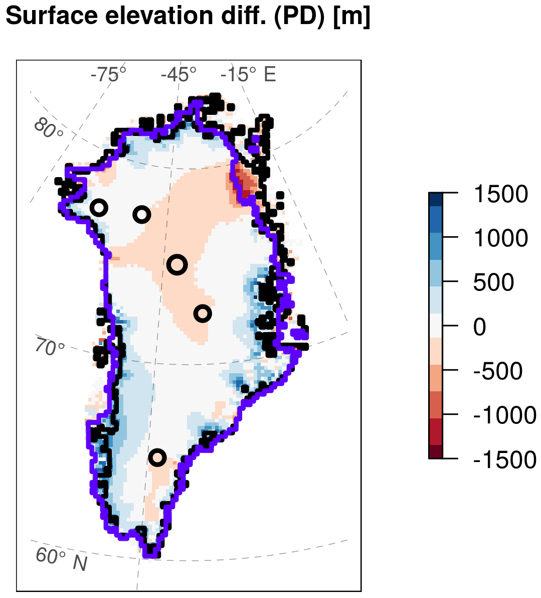
Figure 13Modelled minus observed surface elevation for the present day. Modelled data are taken from the GRISLI-UCM simulation which best estimates the presumed LGM extension (B_ref=1 m a⁻¹ and κ=10 $\mathrm{m}{\mathrm{a}}^{-\mathrm{1}}{\mathrm{K}}^{-\mathrm{1}}$) while the observed surface elevation is taken from Bamber et al. (2013). Purple and black lines represent simulated and observed GrIS extensions, respectively. Black circles indicate the locations of the Camp Century, NEEM, NGRIP, GRIP and Dye3 ice cores (from north to south).

Download