the Creative Commons Attribution 4.0 License.
the Creative Commons Attribution 4.0 License.
 | 22 May 2018
Simulation of the Greenland Ice Sheet over two glacial–interglacial cycles: investigating a sub-ice- shelf melt parameterization and relative sea level forcing in an ice-sheet–ice-shelf model
Sarah L. Bradley
Thomas J. Reerink
Roderik S. W. van de Wal
Michiel M. Helsen
Observational evidence, including offshore moraines and sediment cores, confirm that at the Last Glacial Maximum (LGM) the Greenland ice sheet (GrIS) expanded to a significantly larger spatial extent than seen at present, grounding into Baffin Bay and out onto the continental shelf break. Given this larger spatial extent and its close proximity to the neighbouring Laurentide Ice Sheet (LIS) and Innuitian Ice Sheet (IIS), it is likely these ice sheets will have had a strong non-local influence on the spatial and temporal behaviour of the GrIS. Most previous paleo ice-sheet modelling simulations recreated an ice sheet that either did not extend out onto the continental shelf or utilized a simplified marine ice parameterization which did not fully include the effect of ice shelves or neglected the sensitivity of the GrIS to this non-local bedrock signal from the surrounding ice sheets.
In this paper, we investigated the evolution of the GrIS over the two most recent glacial–interglacial cycles (240 ka BP to the present day) using the ice-sheet–ice-shelf model IMAU-ICE. We investigated the solid earth influence of the LIS and IIS via an offline relative sea level (RSL) forcing generated by a glacial isostatic adjustment (GIA) model. The RSL forcing governed the spatial and temporal pattern of sub-ice-shelf melting via changes in the water depth below the ice shelves.
In the ensemble of simulations, at the glacial maximums, the GrIS coalesced with the IIS to the north and expanded to the continental shelf break to the southwest but remained too restricted to the northeast. In terms of the global mean sea level contribution, at the Last Interglacial (LIG) and LGM the ice sheet added 1.46 and −2.59 m, respectively. This LGM contribution by the GrIS is considerably higher (∼ 1.26 m) than most previous studies whereas the contribution to the LIG highstand is lower (∼ 0.7 m). The spatial and temporal behaviour of the northern margin was highly variable in all simulations, controlled by the sub-ice-shelf melting which was dictated by the RSL forcing and the glacial history of the IIS and LIS. In contrast, the southwestern part of the ice sheet was insensitive to these forcings, with a uniform response in all simulations controlled by the surface air temperature, derived from ice cores.


There have been many ice-sheet modelling studies of the glacial–interglacial evolution of the Northern Hemisphere ice sheets (NHISs) (including the Greenland Ice Sheet (GrIS) and/or Laurentide Ice Sheet (LIS) (Charbit et al., 2007; Greve et al., 1999; Helsen et al., 2013; Ritz et al., 1996; Quiquet et al., 2013) in which there was no expansion of the ice sheet beyond the present-day (PD) coastline during glacial periods. The ice-sheet model in these studies solely modelled the evolution of grounded ice, where the edge of the grounded ice margin was determined by the flotation criterion. However, the wealth of new observational data infers that at glacial maximums the GrIS extended beyond the PD coastline, grounding out onto the continental shelf (Vasskog et al., 2015, and references therein, Sect. 2). This shows there is a mismatch between the observed and the modelled extents.
A review publication by Dutton et al. (2015) stated that the exact magnitude and contribution of the various global ice sheets to global mean sea level (GMSL) during the Last Interglacial (LIG; 130–115 ka BP) is still largely unresolved. From the analysis of far-field sea level records, it is estimated to have reached a peak between 6 and 9 m above PD levels. However, the contribution from the GrIS is poorly constrained and its reconstructed spatial extent highly variable (Vasskog et al., 2015). Estimates from ice-sheet modelling-based studies of the contribution to the LIG highstand range between 0.6 and 3.5 m (Cuffey and Marshall, 2000; Dutton et al., 2015; Helsen et al., 2013; Robinson et al., 2011; Stone et al., 2013). Also, Clark and Tarasov (2014) highlight that closing the Last Glacial Maximum (LGM) GMSL budget is becoming increasingly problematic. This is mostly due to the reduction in the estimated contribution from the Antarctic Ice Sheet (AIS), derived from both modelling and observational studies. In addition, glacial isostatic adjustment (GIA) modelling studies have estimated the contribution of the GrIS to the LGM GMSL budget to be ∼ 5 m (Lecavalier et al., 2014), whereas most ice-sheet modelling-based studies indicate significantly less (typically < 2.5 m; average < 1 m) (Fyke et al., 2011; Letreguilly et al., 1991; Ritz et al., 1996). These lower estimates are possibly caused by restricting the glacial maximum extent to the PD coastline. Consequently, the number of ice-sheet modelling-based studies which simulate a sufficiently large GrIS during glacial periods, both in terms of maximum spatial extent and total contribution to the GMSL budget, are limited, and as a consequence resolving the GrIS GMSL contribution over the last two glacial–interglacial cycles remains problematic. We note, however, the recent Tabone et al. (2018) study, which does address this.
There have been two ice-sheet modelling-based approaches to address the expansion of the grounded ice sheet beyond the PD margin. In the first approach, often referred to as a marine parameterization, ice is permitted to flow and ground beyond the PD coastline to a specified “critical water depth”, regardless of the ice thickness. This critical water depth is either a function of changes in GMSL or constrained by a series of masks reconstructed from observational datasets (Zweck and Huybrechts, 2005). This approach has been adopted in many ice-sheet modelling studies, solving only for grounded ice and reconstructed an extended GrIS during glacial periods (i.e. Huybrechts, 2002; Lecavalier et al., 2014; Simpson et al., 2009). However, rather than the ice sheet evolving freely, it is preconditioned to match with the observational data and does not use any physically based principles.
The second approach includes ice-shelf dynamics in combination with a calculation of sub-ice-shelf melting (SSM). The sub-ice-shelf melt is calculated by a parameterization which is typically based on changes in water depth, estimated using a GMSL forcing. This heuristic approach allows the ice sheet to expand onto the continental shelf but not into the open ocean. There have been a number of publications which applied the second approach using, for instance, the GRISLI ice-sheet model (Ritz et al., 2001). For example, Colleoni et al. (2014) parameterized the SSM as a uniform value in relation to changes in water depth to examine the growth of the NHIS during MIS7 and MIS5. During glacial periods, the reconstructed GrIS grounded across the Nares Strait, the Smith Sound, and out onto the continental shelf to the NE and SW (see Fig. 8 in Colleoni et al., 2014). Although in this reconstruction the ice sheet retreated from the latter two offshore regions (NE and SW) by the LIG minimum (∼ 115 ka BP), it remained grounded across the Nares Strait, which is contrary to the observational data which are reviewed in Sect. 2.
Implicit in both these approaches is that the changes in paleo water depth surrounding the ice sheet are driven by the GMSL forcing, generally derived either from a benthic δ18O record (Lisiecki and Raymo, 2005) or by inverse forward modelling (Bintanja and van de Wal, 2008). However, sea level variations are in fact not simply GMSL (i.e. with no spatial variations), but vary spatially due to numerous processes that dominate over different timescales, with GIA the dominant process on the timescales of this study (Kopp et al., 2015; Rovere et al., 2016).
Table 1Summary of a selection of the observational data which were used to constraint the timing and spatial extent of the grounded ice sheet (Fig. 1).
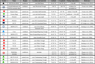
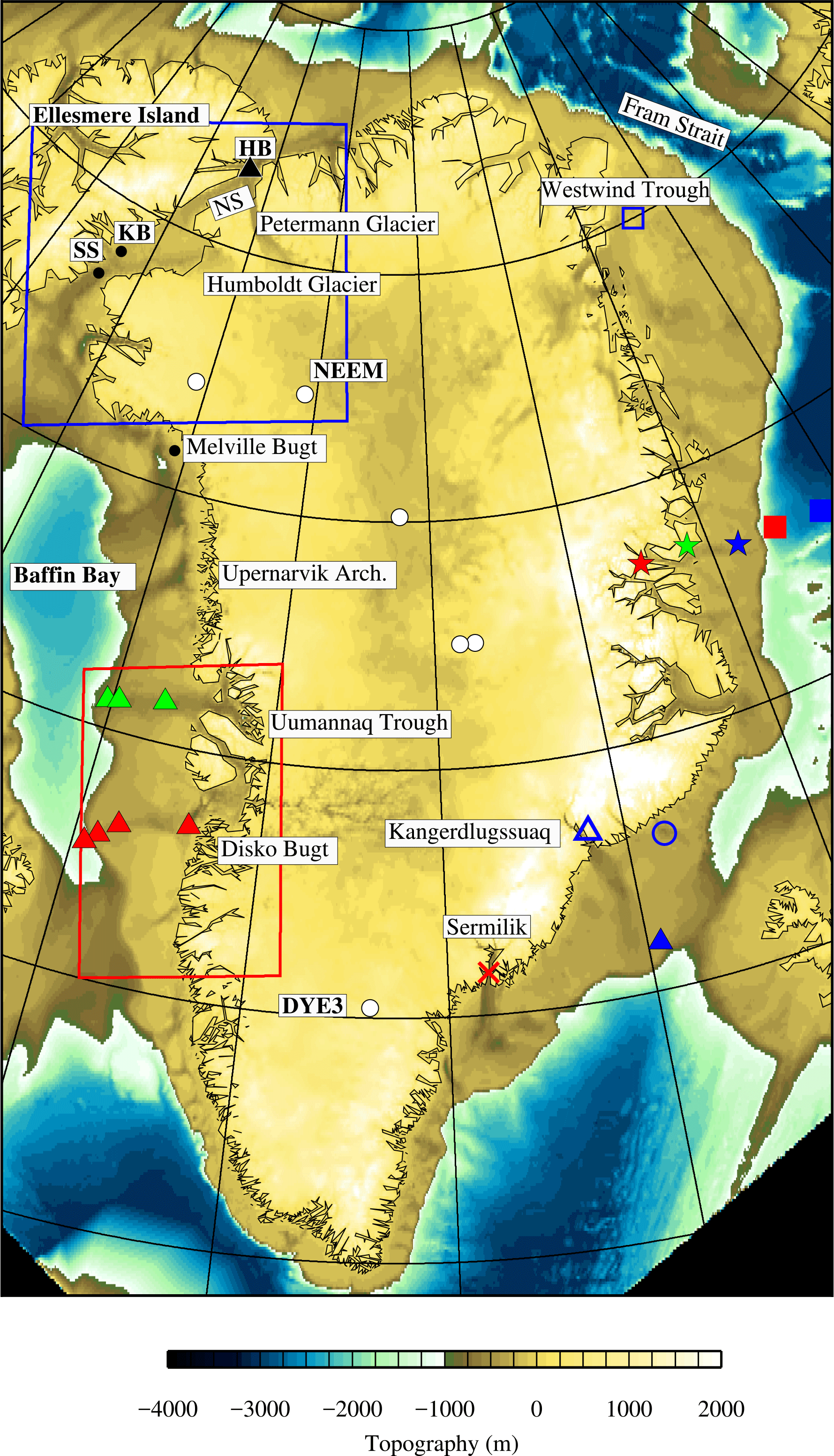
Figure 1Summary of the place names and regions referred to in the main text and locations of observational data. All information describing the symbols and references for the observational data is listed in Table 1. The red and blue boxes highlight the regions shown in Figs. 7 and 8, respectively.
This study advances the second approach, using the ice-sheet–ice-shelf model IMAU-ICE (Sect. 3.1). The GrIS will be simulated over two glacial–interglacial cycles (240 ka BP to the PD), focusing on the parameterizations adopted for SSM (Sect. 3.2). Secondly, to investigate the influence of the spatial and temporal variability in sea level (or water depth) on the GrIS evolution, an offline forcing derived from a GIA model (Sect. 3.3) will be included. The first goal is to investigate if a GrIS larger than that of the PD can be simulated for glacial maximum conditions, which is coherent with the observational data (Sect. 2) and thereby addresses the current mismatch between ice-sheet model and GIA-based GrIS reconstructions. Thirdly, we aim to evaluate the spatial and temporal sensitivity of the GrIS to changes in the SSM and the sea level forcing. Finally, we will address the question of the GrIS contribution to GMSL over the last two glacial–interglacial cycles.
There have been numerous recent publications which have reviewed the wealth of new observational data that can be used to constrain the spatial and temporal history of the GrIS simulated by ice-sheet models (e.g. Funder et al., 2011; Vasskog et al., 2015; Cofaigh et al., 2016) It is not the aim of this study to replicate this information; rather a selection of studies are outlined below which were useful to constrain the ice-sheet model simulations (summarized in Table 1 and Fig. 1).
There are currently six Greenland ice core records (Fig. 1, white circles) that contain evidence of LIG age ice, and so were used to constrain the minimum extent that the ice sheet reached during the LIG (Fig. 1). Only simulations where these six sites remained glaciated at the LIG were considered valid. From the NEEM record (Dahl-Jensen et al., 2013), it is inferred that at 122 ka BP, the surface elevation thinned by 130 ± 300 m. The other five ice core sites remained ice covered, including Dye-3 (Yau et al., 2016). Additionally, analysis of Sr–Nd–Pb isotope ratios in offshore material collected from Erik Drift (Colville et al., 2011) infers that the southern margin retreated to a smaller extent than in the PD but that the ice sheet did not undergo complete deglaciation during the LIG.
Constraining the offshore extent at the Penultimate Glacial Maximum (PGM) or earlier glaciations is complicated as the older geomorphological evidence (i.e. moraines) is overridden by the subsequent readvances. As a consequence, the preservation of offshore sediments is limited. Therefore, we assumed that the ice extent during the PGM and the LGM was equal. The aim with all simulations within the study was to reproduce a spatially expanded grounded ice sheet which reached the constraints given below during these two glacial maximums.
Offshore geomorphological evidence collected from numerous geophysical surveys indicates that the ice sheet grounded out onto the continental shelf (Table 1 and Fig. 1), specifically to the shelf break along the SW, north, and central east at the LGM. This evidence includes moraines, grounding zone wedges (Hogan et al., 2016), large-scale glacial lineations (Cofaigh et al., 2004), and glacio-marine sediments dated and analysed from offshore cores (Jennings et al., 2006). Table 1 provides an overview of the asynchronous nature of the timing of retreat from this expanded glacial maximum towards the PD margin.
Through the expansion of the Petermann and Humboldt glaciers at the NW margin into the Kane and Hall basins and the Nares Strait (Fig. 1), the ice sheet coalesced with the Innuitian Ice Sheet (IIS) at the glacial maximums (LGM or PGM). The grounded ice margin reached south into the north of Baffin Bay and out along the Arctic coastline to the north. Dating one of the few sediment cores from the offshore NW margin (Table 1), Jennings et al. (2011) documented that the retreat of the grounded ice from the Kane and Hall basins initiated after 10.3 ka BP. The margin retreated in an “unzipping manner”, first from the west (Kane Basin) and later to the east (Hall Basin), driven in part by the retreat of IIS back onto Ellesmere Island. The final opening of the connection between the Arctic Ocean and Baffin Bay, via the Nares Strait did not occur until after 9 ka BP, implying that this region was one of the last regions to deglaciate. The retreat of the grounded ice sheet across the Nares Strait and back to the PD margin was a key feature which was used to constrain the simulations, and if ice remained grounded across this margin in the PD, the model simulation was rejected.
Along the NE margin, Evans et al. (2009) concluded that the ice sheet advanced out onto the middle to outer shelf, covering the Westwind Trough (open blue square, Fig. 1). It grounded close to (as indicated by ice-rafted debris (IRD)) but did not extend as far as the Fram Strait, limited by the continental shelf break (see Fig. 1). No dated material was recovered, so the timing is unresolved.
Progressing further south, the lateral extent and timing are better constrained (Table 1) due to the greater availability of data. Retreat from the central east outer shelf initiated by ∼ 15 ka BP (blue star, Fig. 1), stabilizing on the inner shelf at 10 ka BP (green star, Fig. 1), and reaching the PD margin by 7.4 ka BP (red star, Fig. 1) (Cofaigh et al., 2004; Evans et al., 2002). Along the SE margin, the retreat from the outer to inner shelf is highly asynchronous, retreating from the outer Kangerdlugssuaq Trough at ∼ 17.8 ka BP (dark blue triangle, Fig. 1) (earlier than from the central east), reaching the inner fjord by 11.8 ka BP at Kangerdlugssuaq (open blue triangle, Fig. 1) and by 10.8 ka BP at Sermilik (red cross, Fig. 1). It is suggested that the timing of retreat across this region is strongly influenced by the warm incursion of the Irminger current (Dyke et al., 2014).
The SW region of Greenland, around Disko Bugt and the Uumannaq Trough, is one of the more extensively studied regions of the ice sheet, with a range of observational data confirming that the ice sheet grounded out onto the continental shelf break (Cofaigh et al., 2013; Jennings et al., 2014; Sheldon et al., 2016; Winsor et al., 2015). The retreat from the outer shelf (cluster of red triangles, Fig. 1) between 19.3 and 18.6 ka BP is inferred to have been driven by either a change in sea level and/or the ongoing gradual rise in the boreal summer insolation rather than changes in ocean temperatures. The margin stabilized at the middle shelf near the Hellefiske moraine (open red circle, Fig. 1), retreating at 12.24 ka BP and reaching the inner shelf by 10.9 ka BP. The question of whether a change in sea level could initiate such a retreat is just one aspect that the inclusion of a relative sea level (RSL) forcing in this study will address. The retreat from the outer shelf edge in the vicinity of the Uumannaq Fjord (cluster of green triangles, Fig. 1) was later, after 14.9 ka BP, reaching the outer Uumannaq Trough by 10.8 ka BP (Sheldon et al., 2016). Against this background of geological evidence, we evaluated our model results as presented in Sect. 4.
3.1 IMAU-ICE: ice-sheet–ice-shelf model
As the aim of this study is to simulate the expansion onto and retreat from the continental shelf of the GrIS, it is essential to utilize an ice-sheet model which includes the possibility for ice shelves to ground and thereby for the ice sheet to expand beyond the PD margin. To achieve this, we used a 3-D thermomechanical ice-sheet–ice-shelf model IMAU-ICE (previously known as ANICE) (de Boer et al., 2014). For regions of grounded ice, IMAU-ICE uses the commonly adopted shallow-ice approximation (SIA) (Hutter, 1983) to simulate ice velocities in combination with a 3-D thermodynamical approach. For regions of floating ice, the ice-shelf velocities are approximated using the shallow-shelf approximation (SSA) solution (Macayeal, 1989). The model does not accurately solve for grounding line dynamics; rather, the grounding line is defined as the transition between ice-sheet (grounded) and ice-shelf (floating) points using the flotation criterion. The complex marginal topography of Greenland, with narrow troughs with steep gradients, can lead to complications when adopting the usual SSA approach. To address this problem, a 2-D one-sided surface height gradient discretization scheme was included for ice-shelf points neighbouring the grounded line.
In regions within the ice sheet where the basal temperature reaches pressure melting point, the ice sheet is allowed to slide using a Weertman-type sliding law, which relates the sliding velocity (νb) to the basal shear stress (τb) such that
where As is defined as the sliding coefficient, which can be taken as inversely proportional to the bed roughness, z is the reduced normal load, and p and q are spatially uniform constants over the ice-sheet domain. As the roughness at the base of ice sheet is a relatively unknown quantity, a range of sliding coefficients (As) were investigated between 0.04 × 10⁻¹⁰ and 1.8 × 10⁻¹⁰ m8 N−3 yr−1.
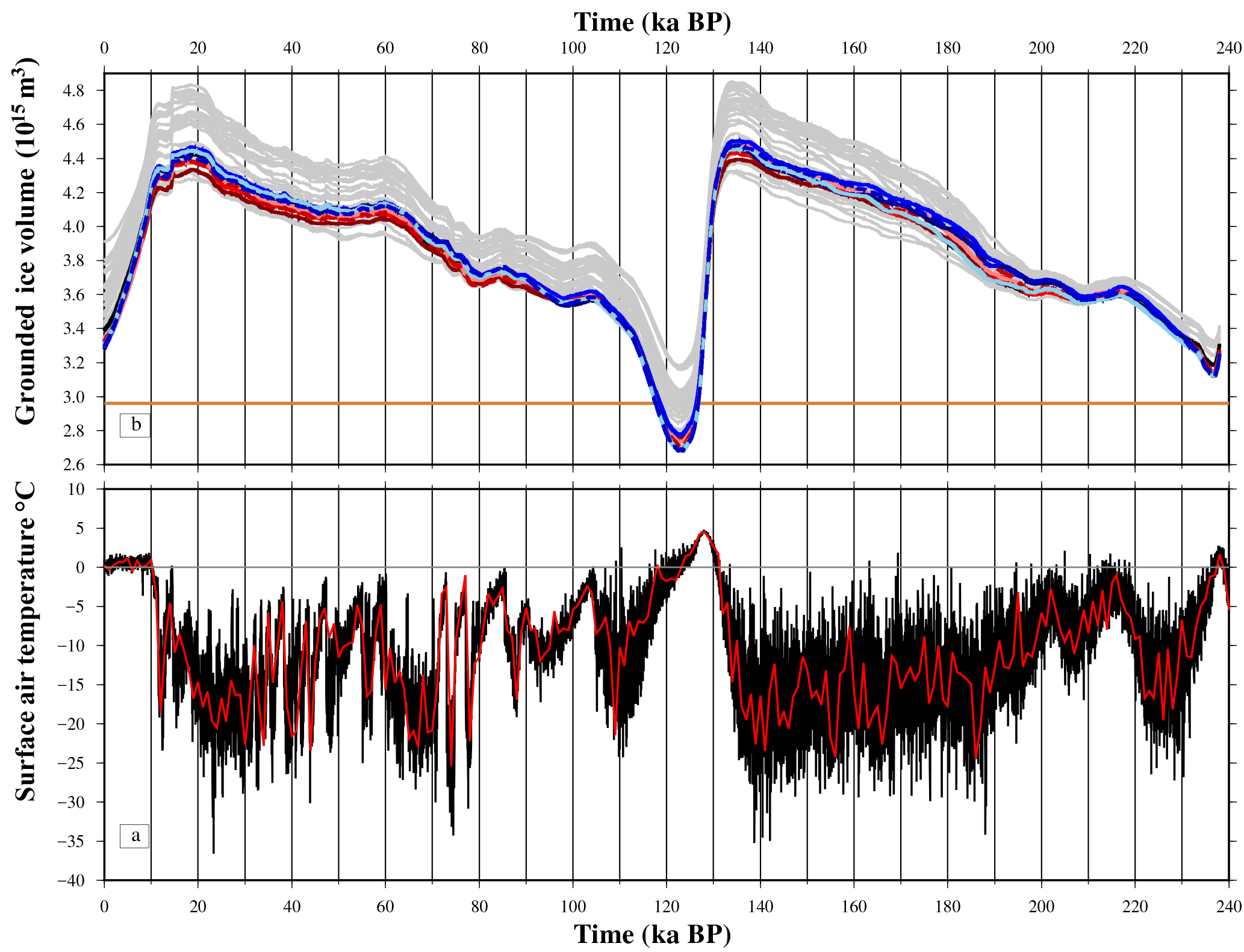
Figure 2(a) Surface air temperature forcing (SAT, ∘C) taken from Helsen et al. (2013), with the solid red line a 2 kyr mean. (b) Grounded ice volume (1015 m3) from the ensemble of simulations (grey lines) and the nine optimum simulations (see Table 3 for colours). The solid orange line marks the present-day ice volume (Bamber et al., 2013).
Present-day input fields of the ice thickness, the surface elevation, and the bed topography are taken from Bamber et al. (2013) with input climate fields (surface mass balance (SMB), refreezing, surface air temperature (SAT)) adapted from the RACMO2 dataset (van Angelen et al., 2014). All these external datasets are interpolated and projected onto the 20 × 20 km ice model grid using the mapping software OBLIMAP2.0 (Reerink et al., 2010, 2016). The adopted OBLIMAP grid projection parameters were λ=371.5, φ=71.8, and α=7.15.
First, IMAU-ICE was run for 100 kyr, under a constant PD climate (using the input climate fields taken from the RACMO2 dataset) to reach an equilibrium state with the aim of replicating the observed PD configuration (Bamber et al., 2013). The sensitivity to the flow enhancement factor (menh, varied between 1 and 5) was investigated for the range of sliding coefficients (As). The resultant ice volume varied over the range of menh and As by ∼ 0.12 × 10¹⁵ m3, with all simulations producing an underprediction of the ice thickness across the centre of the ice sheet and overprediction at the narrow outlet glaciers. Based on this preliminary evaluation, a value of menh=3.5 was used in all simulations. Also, as simulations with an As=1.8 × 10⁻¹⁰ m8 N−3 yr−1 resulted in a significant retreat of the SW margin, the range of sliding coefficients was revised to 0.04 × 10⁻¹⁰ and 1.2 × 10⁻¹⁰ m8 N−3 yr−1 in subsequent simulations. The output of these simulations was used as the initial conditions for the subsequent simulations of the two glacial–interglacial cycles.
Secondly, each simulation was run for 240 kyr using a spatially uniform SAT forcing taken from Helsen et al. (2013) (Fig. 2a), combined with a SSM parameterization (Sect .3.2) and sea level forcing (derived from a GIA model, Sect. 3.3), to simulate the GrIS over the two glacial–interglacial cycles. As there is no GrIS SAT record that extends beyond 128 ka BP, this SAT forcing record was produced by combining the Vostok ice core (Petit et al., 1999) with the GRIP ice core record (Johnsen et al., 2001) using the glacial-index method (Greve, 2005). We note that using a SAT forcing record derived from ice cores will not account for any spatial variability in the SAT during these two glacial–interglacial cycles. The SMB gradient method (Helsen et al., 2012, 2013) was applied at each time step to calculate a new SMB field resulting from this SAT forcing. In this approach, first this uniform temperature forcing (Fig. 2a) is converted into a spatially variable climate-driven surface elevation change using an atmosphere lapse rate of −7.4 K km−1. Second, the SMB gradient fields are calculated based on a linear regression between this new surface elevation field and the mean SMB in an area with a radius of 150 km. With this approach, the spatially uniform temperature forcing (Fig. 2a) can be translated into the spatially varying SMB field and ensures that the local mass balance height feedback is captured. The resultant suite of simulations was evaluated using the observational data defined in Sect. 2.
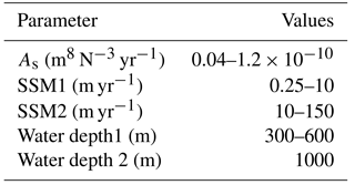
Table 2Range of parameters adopted in the sub-ice-shelf melting (SSM) parameterizations, illustrated in Fig. 3.
3.2 Parameterization of SSM
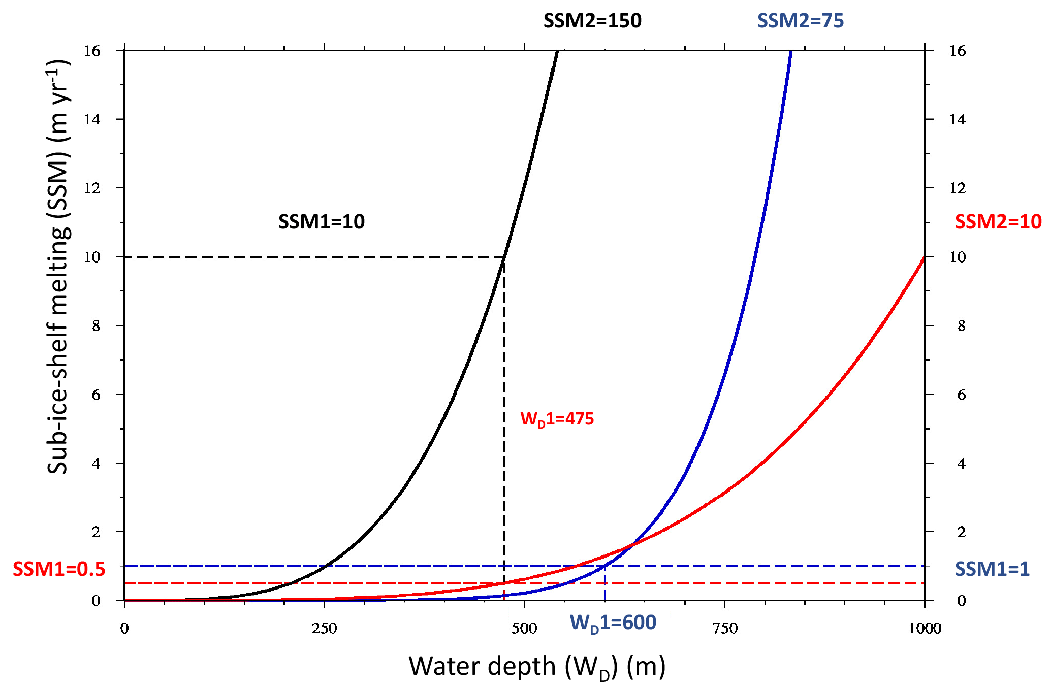
As full physically based models including SSM are still under development, we investigated a SSM parameterization (Fig. 3) primarily based around the assumption that for an increase in paleo water depth (or sea level), there will be a corresponding increase in the amount of SSM. Hence the SSM does not depend on temperature: temperature changes only affect the surface mass balance. In this method, the SSM increases with water depth (WD) by a power law relation with a constant a and exponent m.
In order to conveniently fit this power law through two points (SSM1, WD1) and (SSM2, WD2), we solve
The range of parameter values for SSM1, SSM2, WD1 (water depth1), and WD2 (water depth2) are listed in Table 2, with three examples illustrated in Fig. 3.
3.3 Relative sea level or water depth forcing
In this study, the output from a GIA model is incorporated into IMAU-ICE to examine the influence of spatial and temporal variability in the RSL forcing via the SSM parameterization on the expansion and retreat of the GrIS.
Sea level (or water depth), , can be defined as the vertical distance between the equilibrium ocean surface, the geoid G(θψt), and the solid earth surface R(θψt) (bed topography) (Mitrovica and Milne, 2003). A change in the water depth can result from any vertical deformation in these two surfaces and is defined as
where and are the vertical perturbations in the geoid and solid earth surface at θ co-latitude, ψ eastern longitude, and time t.
In most ice-sheet modelling studies of the GrIS, a spatially uniform, time varying GMSL forcing is used to represent the perturbation in the geoid/ocean surface (G(θψt)), and the deformation of the solid earth (R(θψt)) is calculated using the elastic lithosphere-relaxing asthenosphere (ELRA) method (Le Meur and Huybrechts, 1996). This method only includes the local changes in the solid earth surface resulting from the deglaciation of the GrIS. In reality, the water depth/sea level signal surrounding the GrIS is highly spatially and temporally variable due to the influence of the neighbouring LIS and IIS. On the timescales of this study, the main processes driving this spatial and temporal variability is GIA (Rovere et al., 2016). The variability results from the interplay between the GrIS-driven local changes, as is typical for near-field regions and the non-local changes driven by the LIS and the IIS (Lecavalier et al., 2014). This is because Greenland sits on the resulting forebulge of the LIS. Ideally, the most complete method of incorporating this complex sea level (water depth) signal would be with a coupled ice-sheet–GIA model, as in de Boer et al. (2014). Instead, a simpler alternative method was adopted in this study by coupling offline the output from a GIA model into IMAU-ICE.
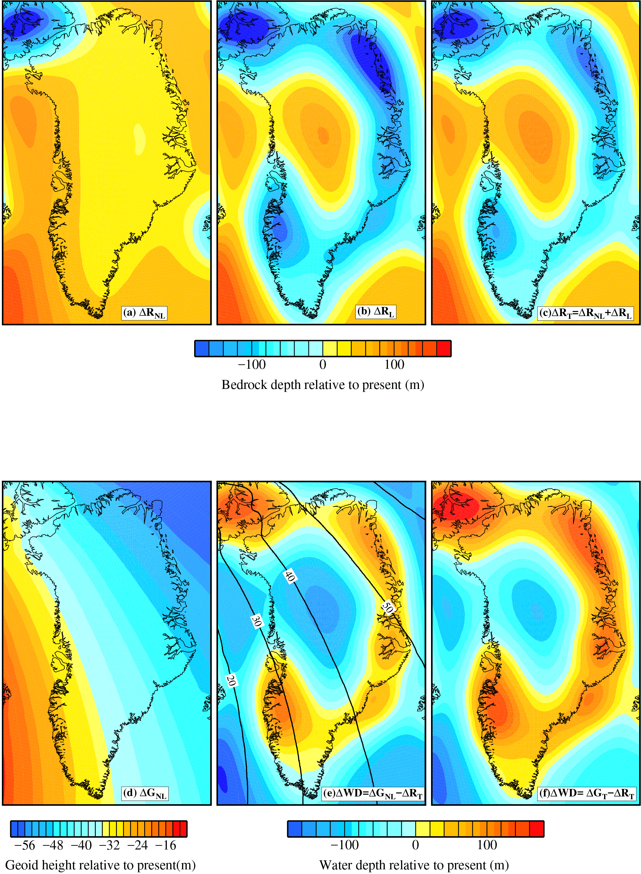
Figure 4Illustration of the various components used within the calculation of the offline RSL forcing at 135 ka BP. Panels (a–c) are the predicted (solid earth deformation) bedrock depth, ΔR: (a) non-local component, ΔRNL (No GrIS); (b) local component, ΔRL (GrIS only); and (c) total signal. ΔRT (d) Predicted non-local geoid signal, ΔGNL (No GrIS). The predicted water depth (WD) signal is illustrated for (e) ΔGNL−ΔRT: combination of total predicted bedrock depth and non-local geoid. It is this signal which is used within all simulations. Contoured is the local signal, ΔGL, which is not included. (f) Total water depth signal, ΔWD. See text for extra details.
Table 3Set of optimum parameters which resulted in a growth beyond the PD margin during glacial maximums (PGM and LGM) and a retreat by the present day (PD). Note that WD2 is constant in all simulations (1000 m). The simulation highlighted in grey is shown in Fig. 5. The timing of the retreat across the Nares Strait for two interglacials is given in ka BP: PGM–LIG and LGM–PD, along with the total global mean sea level (GMSL) contribution from the GrIS only for the Last Interglacial (LIG) and the Last Glacial Maximum (LGM). The GMSL was calculated using the simulated ice volume.
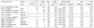
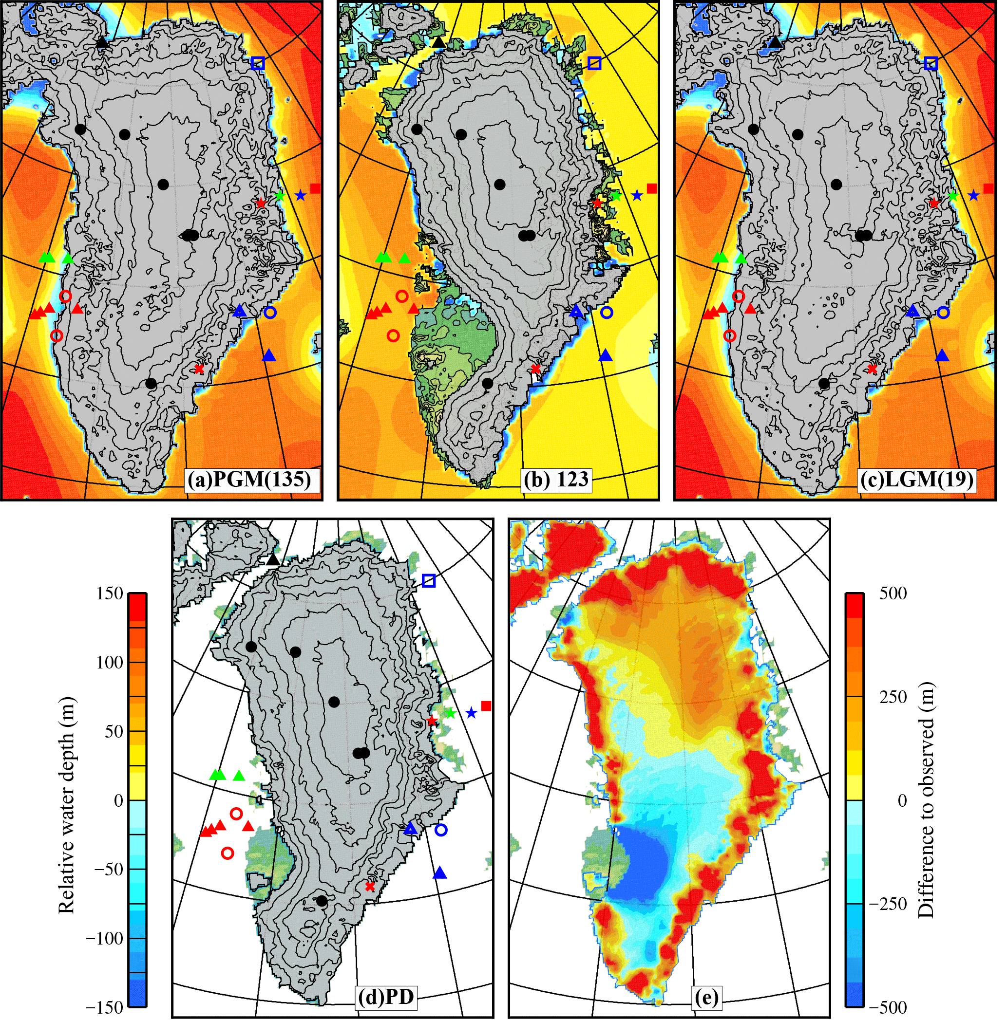
Figure 5Simulated extent of the grounded ice sheet and relative water depth using the parameters highlighted in Table 3 (AvAs+ AvSSM1) at four time periods: (a) Penultimate Glacial Maximum (PGM), 135 ka BP; (b) Last Interglacial (LIG) minimum, 123 ka BP; (c) Last Glacial Maximum (LGM), 19 ka BP; and (d) the present day (PD). Panel (e) is the difference in the present-day surface elevation (relative to the observed surface elevation; Bamber et al., 2013), where positive value indicates an overprediction. The black circles mark the location of the GrIS ice core sites. Observed data constraining the timing of retreat is summarized in Table 1. Note that the colour bar extended beyond (±) 150. Small floating ice shelves formed at the edge of the grounded ice sheet, but these are not shown.
To incorporate the output from the GIA model, first Eq. (4) was decomposed into (a) a local (subscript “L”) signal, driven by changes in the GrIS (ΔGL,ΔRL) and (b) a non-local signal (subscript NL) driven by the influence of all other ice sheets, primarily the LIS (ΔGNL,ΔRNL).
Hence the relationship for the change in water depth is written as
In order to solve this relationship, a GIA model was used to calculate the non-local contributions (ΔGNL (Fig. 4d) and ΔRNL (Fig. 4a)). This model has three key input components: a reconstruction of Late Pleistocene ice-sheet history (Peltier, 2004), an earth model that simulates the solid earth deformation due to changes in the surface mass redistribution between the oceans and ice sheets (Peltier, 1974), and a model of sea level change (Farrell and Clark, 1976). The sea level model included perturbations to the rotation vector (Milne and Mitrovica, 1998; Mitrovica et al., 2001, 2005), time-dependent shoreline migration, and an accurate treatment of sea level change in areas characterized by ablating marine-based ice (Kendall et al., 2005; Mitrovica and Milne, 2003).
To run the GIA model over the two glacial–interglacial cycles (240 ka to the PD) to produce the non-local signals, an input global ice reconstruction is required which reproduces the spatial and temporal history of all global ice sheets, apart from the GrIS during this interval. As a basis for this reconstruction, the ICE5G global ice model (Peltier, 2004) was adopted, which extends from 122 ka BP to the PD: one glacial–interglacial cycle. As the history for two glacial–interglacial cycles was required, the ice history over the 122 kyr was duplicated to represent the previous glacial–interglacial cycles (240 ka to 122 ka BP), resulting in an ice-sheet reconstruction from 240 ka BP to the PD. The GrIS component was removed from the ICE5G global ice model to produce the final non-local input ice history. The adopted earth model is characterized by a 96 km lithosphere and an upper and lower mantle viscosity of 5 × 10²⁰ Pa s and 1 × 10²² Pa s, respectively. These viscosity parameters fall approximately within the middle of the range of values commonly inferred. Using this input ice history and earth model the GIA model was run offline to produce the non-local geoid and deformation fields (ΔGNL (Fig. 4d) and ΔRNL (Fig. 4a)).
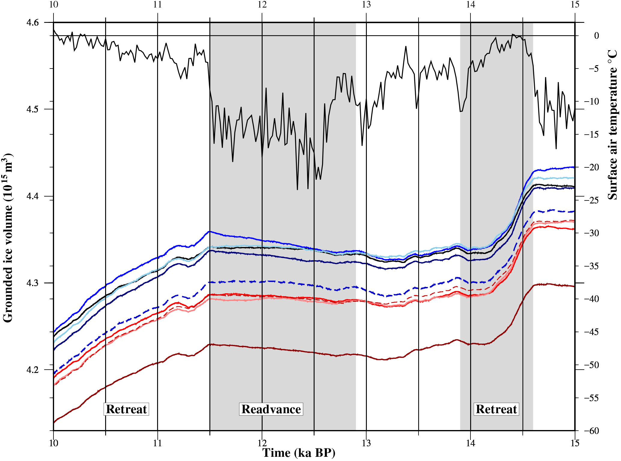
Figure 6Comparison of the grounded ice volume (1015 m3) from the nine optimum simulations (see Table 3 for colours) and the surface air temperature forcing (∘C) (black line; Fig. 2a) from 15 to 10 ka BP. Highlighted are the timings of the retreat–readvance–retreat of the SW margin (red box; Fig. 1), the spatial pattern of which is illustrated for AvAs+AvSSM1 (light red line) in Fig. 7. Results for the NW are illustrated in Fig. 8.
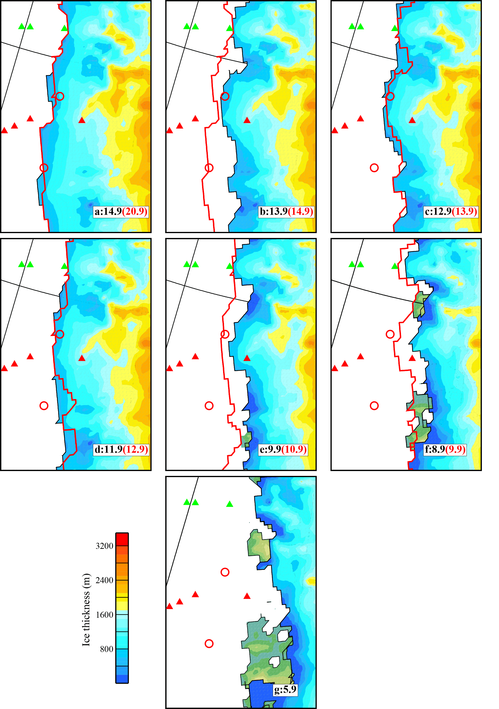
Figure 7Retreat of the grounded ice sheet along the SW margin (region bounded by the red box in Fig. 1) for AvAs+AvSSM1 (ka BP). The red contour marks the edge of the grounded ice sheet at an earlier time step (given in red): (a) 14.9 (20.9), (b) 13.9 (14.9), (c) 12.9 (13.9), (d) 11.9 (12.9), (e) 9.9 (10.9), (f) 8.9 (9.9), and (g) 5.9. There is minimal change between the extent at 5.9 and the present day. Observed data constraining the timing of retreat are summarized in Table 1. Small floating ice shelves formed at the edge of the grounded ice sheet, but these are not shown.

Figure 8Examples of the influence of the choice of SSM parameter and RSL forcing on the spatial and temporal retreat pattern across the NW margin (region bounded by the blue box in Fig. 1). Panels (a) and (b) compare the grounded ice-sheet extent between two simulations AvAs_lowSSM1-0.5_shallow and HighAs_lowSSM1-0.25 to highlight the impact of the choice of As in controlling the onset of the LGM-to-PD retreat. The red contour marks the edge of the grounded ice sheet at an earlier time step. Panels (c) and (d) illustrate the difference in the simulated water depth and maximum grounded ice-sheet extent (shaded grey region) between simulations AvAs+ AvSSM1 and AvAs+ AvSSM1_redSSM2. The main difference between these two simulations is the choice of SSM2 as 100 m yr−1 (AvAs+ AvSSM1) compared to 75 m yr−1 (AvAs+ AvSSM1_redSSM2).
As the GIA model is used to produce the non-local components, the local fields (ΔRL, ΔGL) driven by the GrIS are still required to solve Eq. (5). The locally driven changes in the solid earth surface, ΔRL, were calculated internally within IMAU-ICE, using the ELRA method (Le Meur and Huybrechts, 1996) (Fig. 4b). This local field (ΔRL) is combined with ΔRNL(from the GIA model) to calculate the total deformation of the solid earth surface ΔRT (Fig. 4c). This is combined with the non-local geoid signal, GNL (Fig. 4d), to produce the final ΔWD, which is used to force the ice-sheet model at each time step (Fig. 4e).
Referring back to Eq. (5), using this method results in the following revised equation for ΔWD.
However, comparing Eqs. (6) to (5), it is evident that the local geoid, ΔGL, is not calculated using this approach and can be defined as a missing signal. To calculate this local geoid signal, ΔGL, would require solving the sea level equation (as within the GIA model; see de Boer et al., 2014) resulting from these local GrIS-driven changes within IMAU-ICE, which is not possible within the adopted approach. To estimate the magnitude of this missing local geoid signal, the difference between the total signal, which is calculated using the GIA model (Fig. 4f, derived from Eq. 5) and the signal as obtained from Eq. (6) (Fig. 4e) was calculated. This difference is small (contoured in Fig. 4e) but is a shortcoming of the modelling that is accepted given the simplicity of the other components of the model. It is noted that this approach, for example, neglects feedbacks between changes in the sea level and the marine-based ice and the stabilizing influence this may have on the evolution of the ice shelves (de Boer et al., 2014; Gomez et al., 2010).
As Fig. 4a illustrates, at the PGM there is a significant non-local deflection in the solid earth surface. Across Ellesmere Island and NW Greenland, the LIS and IIS produce significant subsidence of up to 200 m. Central Greenland and Baffin Bay are elevated by up to 100 and 30 m, respectively, due to the influence of the forebulge. In contrast, the non-local geoid signal is much smaller, with a range of ∼ 40 m (Fig. 4d). Comparing these two signals, it is apparent that the deflection of the solid earth surface will be the main contributor to driving changes in water depth/sea level in this study (Fig. 4e and f).
There were only nine combinations of SSM1, SSM2, WD1, and As from the ensemble of simulations that resulted in glacial–interglacial retreat over the two glacial–interglacial cycles (Table 3) and fulfilled the conditions defined in Sect. 2. Two additional simulations are included in Table 3 (LowAs_lowSSM1-0.25_deep and HighAs_highSS1) which only resulted in a glacial–interglacial expansion between the LGM and the PD, one glacial–interglacial cycle. The spatial extent at selected time periods is illustrated for one example simulation in Fig. 5.
At the glacial maximums (PGM and LGM) the simulated ice sheet reached the inferred observational limits along the northern and eastern margin (Fig. 5a and c); however, at the SW margin (see red and green triangles, Fig. 5a and c) the ice sheet remains too restricted, possibly related to too strong a mass balance height feedback in this region. The average LGM GMSL contribution is −2.59 m, which is still ∼ 50% smaller than estimates from GIA modelling-based studies (i.e. Lecavalier et al., 2014). Therefore, closing the LGM GMSL budget remains problematic.
The simulated LIG minimum extent in all nine simulations complied with the spatial limits inferred from the LIG ice core data, with a thinning at NEEM (∼ 250 m) and a moderate inland retreat of the SW margin, but with Dye-3 remaining covered with grounded ice (Fig. 5b). The average LIG GMSL contribution was 1.46 m (Table 3), which lies within the most recent estimated range of between 0.6 and 3.5 m (Dutton et al., 2015). At the PD, the SW margin has retreated too far inland (Fig. 5d and e) and there is a pronounced overthickening (up to 500 m) along most of the coastline (Fig. 5e). Preliminary simulations concluded that increasing the resolution to 10 × 10 km reduced this misfit, but a more detailed modelling of outlet glaciers at scales down to kilometres is likely needed to fully resolve this misfit.
There is an evident correlation between the temporal variability of SAT forcing and the total ice volume in all simulations, the periods of maximum ice volume (PGM, LGM) corresponding with the minimum in SAT and vice versa (Fig. 2). This would imply that the timings of the glacial–interglacial variations are strongly dependent on the adopted SAT forcing. However, there is a spatially variable response between the NW and SW margins which implies that the two regions respond regionally to a different forcing mechanism or at least a different timing of the same mechanism. Therefore, the interplay between the SAT and RSL forcing and the spatial and temporal variability in these two margins is examined in greater detail for the last 20 kyr.
It is evident from Fig. 6 that there is minimal variation in total ice volume and spatial extent between the nine simulations from the LGM (∼ 19 ka BP) to 14.6 ka BP (Fig. 7a). This corresponds to a period of relatively stable SAT ∼ −15∘ C and minimal variations in the non-local RSL forcing (either the predicted bedrock depth or sea surface height (similar to that illustrated in Fig. 4)) due to only minor changes in the glacial history of the LIS (Peltier, 2004). Following this, there are three time periods (highlighted in Fig. 6) where changes in the ice volume and SAT correlate with a significant retreat/readvance along the SW, SE, and to a lesser extent NE margins (Fig. 7), but with the NW margin remaining stable. Between 14.6 ka BP (Fig. 6) and ∼ 13.9 ka BP there is a rapid retreat in the grounded SW margin (Figs. 6, 7a–b) and a fall in ice volume of ∼ 1.0 × 10¹⁵ m3 (∼ 0.24 m GMSL). This coincides with a warming (∼ 10 ∘C; Fig. 6) and a strong non-local RSL signal due to a significant retreat of the LIS. As the LIS deglaciated, it produced a non-local subsidence of the bedrock (Fig. 4a) across this margin, increasing the water depth and in turn the SSM. Following this retreat, there is a ∼ 1 kyr stillstand in the grounded ice extent (Fig. 7c), during which there is a slow gradual cooling (Fig. 6). From ∼ 12.9 to 11.5 ka BP (Figs. 6, 7d), during a period of pronounced cooling (∼ 15 ∘C, Fig. 6), the ice sheet readvances along the SW margin, producing a small increase in total ice volume (largest in simulations with high As), with the main period of retreat commencing at 11.5 ka BP at the onset of the sharp rise in SAT (∼ 12 ∘C). This readvance (12.9–11.5 ka BP) coincides with the ongoing large non-local RSL signal (subsidence) which in turn results in an increase in SSM. This interplay implies that changes in the SSM (driven by the RSL signal) have only a secondary influence on the dynamics of the SW margin. This is emphasized by the minimal variations in the behaviour of the SW margins between the nine final simulations. In Sect. 2, from analysis of observational data, it was inferred that the retreat from this margin may, in part be driven by the changes in RSL forcing. The simulations carried out in this study suggest that this is not the case, with the retreat driven primarily by SAT forcing.
The spatial and temporal behaviour of the NW margin (blue box, Fig. 1) in all nine simulations (Table 3) is highly variable, correlating with changes in the SSM, driven by the non-local and local RSL forcing. There is minimal correlation with the timings of the SAT forcing. In all simulations, the timing of final deglaciation of the NW margin was too late compared to observations (∼ 10–9 ka BP), but the spatial pattern as inferred by Jennings et al. (2011) of a retreat initiated first at the western margin and later to the east is replicated. This is due to the faster ice velocity within the narrow outlet fjords to the west, i.e. in the Humboldt Glacier, which feed into the grounded ice sheet across the Kane Basin (relative to the eastern grounded margin across the Hall Basin). The initiation of this retreat (at 8.9 ka BP at the earliest, Table 3) was controlled in part by the timing of the final deglaciation of the LIS within the ICE5G global ice model (Peltier, 2004) but also by the influence of the IIS which was simulated within IMAU-ICE. In ICE5G, the LIS retreats across Hudson Bay at 10 ka BP with complete deglaciation of the high Arctic by ∼ 8 ka BP. This drives the onset of the non-local subsidence of the solid earth surface (bedrock) (ΔRNL) across this region (Fig. 4a and c), as the LIS forebulge collapses. It is noted that changes in the choice of earth model and/or the spatial and temporal deglaciation history of the LIS during this final deglaciation interval will of course directly impact on the timing of the GrIS retreat.
The non-local influence of the IIS (which develops across Ellesmere Island) also strongly governed the timing of the retreat of the NW margin, which can be seen by comparing the results from two simulations: HighAs_lowSSM1-0.25 to HighAs_lowSSM1 (see Table 3). It could be assumed – given the lower SSM1 (0.25 m yr−1 compared to 0.5 m yr−1) in HighAs_lowSSM1-0.25 which results in a lower SSM close to the edge of the grounded ice margin – that the onset of the retreat would be later. However, the retreat is in fact 1 kyr earlier. In this simulation (HighAs_lowSSM1-0.25), the IIS is considerably thicker (> 1500 m), increasing the subsidence of the solid earth surface (bedrock) (due to the increased ice loading) and the water depth and in turn producing a higher SSM, which drives the earlier deglaciation. This highlights the influence of the IIS on controlling the deglaciation of the GrIS across this region.
The amount of basal sliding (via the choice of As) also influences the timing of the onset of the NW margin retreat, with a lower amount of basal sliding generally promoting an earlier retreat (comparing the average As (labelled AvAs) simulations to the High As simulations (labelled HighAs) in Table 3). This is examined in detail for two simulations: AvAs_lowSSM1-0.5_shallow and HighAs_lowSSM1-0.25 (Fig. 8a and b). The retreat is initiated 5 kyr earlier in the simulation with a lower As value (AvAs_lowSSM1-0.5_shallow). The earlier onset of the retreat with a lower As is due in part to the more restricted and thinner grounded ice sheet across the NW margin, so there is a smaller volume of ice to retreat (compare the red contours in Fig. 8a and b), and is also due to the different SSM parameters. In AvAs_lowSSM1-0.5_shallow the combination of a higher SSM1 (0.5 m yr−1 compared to 0.25 m yr−1) and a shallower WD1 (300 m compared to 475 m) results in SSM that is higher at all water depths. It is this combination of a higher SSM with the lower As which drives the earlier onset of retreat and more restricted glacial maximum extent (Fig. 8a).
The SSM at deeper water depths (> WD1), controlled by SSM2, also strongly influences the behaviour of the NW margin via the impact on the PGM-to-LIG glacial history, i.e. the first glacial–integlacial cycle. Fig. 8c and d compare the difference in the simulated water depth between two simulations (AvAs+AvSSM1 and AvAs+AvSSM1_redSSM2) where the SSM2 is reduced by 25 m yr−1 (from 100 to 75 m yr−1). It could be assumed, given the reduction in SSM at deeper water depth, that the retreat would be later. However, the onset of retreat is 2 kyr earlier (8.9 ka BP compared to 6.9 ka BP). This is due to the influence of the PGM-to-LIG glacial history (first glacial–interglacial cycle) on the dynamics of the LGM-to-PD retreat (second glacial–interglacial cycle). In the AvAs+AvSSM1_redSSM2 simulation, during the first advance of the ice sheet, the lower SSM at water depths > 400 m results in a thicker ice sheet across the Nares Strait and eastern Ellesmere Island (part of the IIS). This increases the bedrock subsidence and the water depth (Fig. 8c) resulting in a higher SSM surrounding the retreated ice margin during the subsequent glacial–interglacial cycle (after the LIG minimum). This higher SSM restricts the maximum spatial extent that the grounded ice margin reaches during the subsequent LGM-to-PD glacial–interglacial cycle (compare Fig. 8d to a and b). Therefore, with a smaller ice extent, surrounded by a region of higher SSM, this induces an earlier onset of retreat.
In this study using the ice-sheet–ice-shelf model, IMAU-ICE, the evolution of the GrIS over the two most recent glacial–interglacial cycles (240 ka BP to the PD) was investigated. The sensitivity of the spatial and temporal behaviour of the ice sheet to an offline RSL forcing, generated by a GIA model was incorporated. Through this, the influence of the glacial history of the LIS and IIS was explored. This RSL forcing governed the spatial and temporal pattern of SSM via changes in the water depth below the ice shelves that developed around the ice sheet. The SSM was parameterized in relation to the water depth, where for an increase in water depth, the SSM increased. We note that we do not investigate the influence of these two ice sheets (LIS and IIS) on the atmospheric circulation; there was no climate model used within our study.
At the LIG minimum, all of the LIG ice cores remain ice covered, with a ∼ 250 m thinning at NEEM and an inland retreat of the SW margin, contributing 1.46 m to the LIG highstand, a reduction of ∼ 0.7 m relative to previous studies. At the glacial maximums, the ice sheet expanded offshore to coalesce with the IIS, reaching the Smith Sound at the north of Baffin Bay as well as the continental shelf along the SW. However, it is still too restricted to the NE. A LGM GMSL contribution of −2.59 m is considerably higher than most previous studies (∼ 1.26 m), but closing the LGM GMSL budget remains problematic.
The temporal response of the SW margin was primarily controlled by the adopted SAT forcing (taken from ice core records). The RSL forcing and the choice of SSM parameterization were of secondary influence. However, the inclusion of the RSL forcing improved the reconstructed PD GrIS by reducing an underprediction along the SW margin (relative to observations). Conversely, the NW margin, where the ice sheet coalesced with the IIS, was relatively insensitive to the imposed SAT forcing. Instead the spatial and temporal response was controlled by variations in the resultant SSM patterns that are driven by the variability in the RSL forcing and the glacial history of the LIS and IIS. The combined RSL and temperature changes generate a highly variable temporal response, where optimum parameters were found to be a sliding coefficient As in the range of 1.0 × 10⁻¹⁰ to 1.2 × 10⁻¹⁰ m8 N−3 yr−1; a relatively low SSM close to the grounded ice margin to allow glacial expansion; and a higher SSM at deeper water depths to promote interglacial retreat.
The IMAU-ICE model is part of the ICEDYN package. The code used in this study is based on the ICEDYN SVN revision 2515. OBLIMAP is an open-source package which is available at https://github.com/oblimap/oblimap-2.0 (Reerink, 2018).
Output from all simulations, including the GIA model used for the RSL forcing used within this study, is available from Sarah L. Bradley upon request.
The authors declare that they have no conflict of interest.
Sarah L. Bradley and Thomas J. Reerink acknowledge support from the
Netherlands Earth System Science Centre (NESSC), which is financially
supported by the Ministry of Education, Culture and Science (OCW).
Michiel M. Helsen was supported by The Netherlands Polar Programme (NPP) of
the Earth and Life Sciences division of The Netherlands Organisation for
Scientific Research (NWO/ALW).
Edited by:
David Thornalley
Reviewed by: Ilaria Tabone and one anonymous
referee
Bamber, J. L., Griggs, J. A., Hurkmans, R., Dowdeswell, J. A., Gogineni, S. P., Howat, I., Mouginot, J., Paden, J., Palmer, S., Rignot, E., and Steinhage, D.: A new bed elevation dataset for Greenland, The Cryosphere, 7, 499–510, https://doi.org/10.5194/tc-7-499-2013, 2013.
Bintanja, R. and van de Wal, R. S. W.: North American ice-sheet dynamics and the onset of 100,000-year glacial cycles, Nature, 454, 869–872, https://doi.org/10.1038/nature07158, 2008.
Charbit, S., Ritz, C., Philippon, G., Peyaud, V., and Kageyama, M.: Numerical reconstructions of the Northern Hemisphere ice sheets through the last glacial-interglacial cycle, Clim. Past, 3, 15–37, https://doi.org/10.5194/cp-3-15-2007, 2007.
Clark, P. U. and Tarasov, L.: Closing the sea level budget at the Last Glacial Maximum, P. Natl. Acad. Sci. USA, 111, 15861–15862, https://doi.org/10.1073/pnas.1418970111, 2014.
Cofaigh, C. Ó., Dowdeswell, J. A., Evans, J., Kenyon, N. H., Taylor, J., Mienert, J., and Wilken, M.: Timing and significance of glacially influenced mass-wasting in the submarine channels of the Greenland Basin, Mar. Geol., 207, 39–54, https://doi.org/10.1016/j.margeo.2004.02.009, 2004.
Cofaigh, C. O., Dowdeswell, J. A., Jennings, A. E., Hogan, K. A., Kilfeather, A., Hiemstra, J. F., Noormets, R., Evans, J., McCarthy, D. J., Andrews, J. T., Lloyd, J. M., and Moros, M.: An extensive and dynamic ice sheet on the West Greenland shelf during the last glacial cycle, Geology, 41, 219–222, https://doi.org/10.1130/g33759.1, 2013.
Cofaigh, C. O., Briner, J. P., Kirchner, N., Lucchi, R. G., Meyer, H., and Kaufman, D. S.: PAST Gateways (Palaeo-Arctic Spatial and Temporal Gateways): Introduction and overview, Quaternary Sci. Rev., 147, 1–4, https://doi.org/10.1016/j.quascirev.2016.07.006, 2016.
Colleoni, F., Masina, S., Cherchi, A., Navarra, A., Ritz, C., Peyaud, V., and Otto-Bliesner, B.: Modeling Northern Hemisphere ice-sheet distribution during MIS 5 and MIS 7 glacial inceptions, Clim. Past, 10, 269–291, https://doi.org/10.5194/cp-10-269-2014, 2014.
Colville, E. J., Carlson, A. E., Beard, B. L., Hatfield, R. G., Stoner, J. S., Reyes, A. V., and Ullman, D. J.: Sr-Nd-Pb Isotope Evidence for Ice-Sheet Presence on Southern Greenland During the Last Interglacial, Science, 333, 620–623, 2011.
Cuffey, K. M. and Marshall, S. J.: Substantial contribution to sea-level rise during the last interglacial from the Greenland ice sheet, Nature, 404, 591–594, https://doi.org/10.1038/35007053, 2000.
Dahl-Jensen, D., Albert, M. R., Aldahan, A., Azuma, N., Balslev-Clausen, D., Baumgartner, M., Berggren, A. M., Bigler, M., Binder, T., Blunier, T., Bourgeois, J. C., Brook, E. J., Buchardt, S. L., Buizert, C., Capron, E., Chappellaz, J., Chung, J., Clausen, H. B., Cvijanovic, I., Davies, S. M., Ditlevsen, P., Eicher, O., Fischer, H., Fisher, D. A., Fleet, L. G., Gfeller, G., Gkinis, V., Gogineni, S., Goto-Azuma, K., Grinsted, A., Gudlaugsdottir, H., Guillevic, M., Hansen, S. B., Hansson, M., Hirabayashi, M., Hong, S., Hur, S. D., Huybrechts, P., Hvidberg, C. S., Iizuka, Y., Jenk, T., Johnsen, S. J., Jones, T. R., Jouzel, J., Karlsson, N. B., Kawamura, K., Keegan, K., Kettner, E., Kipfstuhl, S., Kjaer, H. A., Koutnik, M., Kuramoto, T., Kohler, P., Laepple, T., Landais, A., Langen, P. L., Larsen, L. B., Leuenberger, D., Leuenberger, M., Leuschen, C., Li, J., Lipenkov, V., Martinerie, P., Maselli, O. J., Masson-Delmotte, V., McConnell, J. R., Miller, H., Mini, O., Miyamoto, A., Montagnat-Rentier, M., Mulvaney, R., Muscheler, R., Orsi, A. J., Paden, J., Panton, C., Pattyn, F., Petit, J. R., Pol, K., Popp, T., Possnert, G., Prie, F., Prokopiou, M., Quiquet, A., Rasmussen, S. O., Raynaud, D., Ren, J., Reutenauer, C., Ritz, C., Rockmann, T., Rosen, J. L., Rubino, M., Rybak, O., Samyn, D., Sapart, C. J., Schilt, A., Schmidt, A. M. Z., Schwander, J., Schupbach, S., Seierstad, I., Severinghaus, J. P., Sheldon, S., Simonsen, S. B., Sjolte, J., Solgaard, A. M., Sowers, T., Sperlich, P., Steen-Larsen, H. C., Steffen, K., Steffensen, J. P., Steinhage, D., Stocker, T. F., Stowasser, C., Sturevik, A. S., Sturges, W. T., Sveinbjornsdottir, A., Svensson, A., Tison, J. L., Uetake, J., Vallelonga, P., van de Wal, R. S. W., van der Wel, G., Vaughn, B. H., Vinther, B., Waddington, E., Wegner, A., Weikusat, I., White, J. W. C., Wilhelms, F., Winstrup, M., Witrant, E., Wolff, E. W., Xiao, C., Zheng, J., and Community, N.: Eemian interglacial reconstructed from a Greenland folded ice core, Nature, 493, 489–494, https://doi.org/10.1038/nature11789, 2013.
de Boer, B., Stocchi, P., and van de Wal, R. S. W.: A fully coupled 3-D ice-sheet-sea-level model: algorithm and applications, Geosci. Model Dev., 7, 2141–2156, https://doi.org/10.5194/gmd-7-2141-2014, 2014.
Dutton, A., Carlson, A. E., Long, A. J., Milne, G. A., Clark, P. U., DeConto, R., Horton, B. P., Rahmstorf, S., and Raymo, M. E.: Sea-level rise due to polar ice-sheet mass loss during past warm periods, Science, 349, https://doi.org/10.1126/science.aaa4019, 2015.
Dyke, L. M., Hughes, A. L. C., Murray, T., Hiemstra, J. F., Andresen, C. S., and Rodés, Á.: Evidence for the asynchronous retreat of large outlet glaciers in southeast Greenland at the end of the last glaciation, Quaternary Sci. Rev., 99, 244–259, https://doi.org/10.1016/j.quascirev.2014.06.001, 2014.
Evans, J., Dowdeswell, J. A., Grobe, H., Niessen, F., Stein, R., Hubberten, H. W., and Whittington, R. J.: Late Quaternary sedimentation in Kejser Franz Joseph Fjord and the continental margin of East Greenland, Geol. Soc., London, Special Publications, 203, 149–179, 2002.
Evans, J., Cofaigh, C. O., Dowdeswell, J. A., and Wadhams, P.: Marine geophysical evidence for former expansion and flow of the Greenland Ice Sheet across the north-east Greenland continental shelf, J. Quaternary Sci., 24, 279–293, https://doi.org/10.1002/jqs.1231, 2009.
Farrell, W. E. and Clark, J. A.: Post Glacial Sea-Level, Geophys. J. Roy. Astr. S., 46, 647–667, 1976.
Funder, S., Kjeldsen, K. K., Kjær, K. H., and Ó Cofaigh, C.: Chapter 50 – The Greenland Ice Sheet During the Past 300,000 Years: A Review, in: Developments in Quaternary Sciences, edited by: Ehlers, J., Gibbard, P. L., and Hughes, P. D., Elsevier, 699–713, 2011.
Fyke, J. G., Weaver, A. J., Pollard, D., Eby, M., Carter, L., and Mackintosh, A.: A new coupled ice sheet/climate model: description and sensitivity to model physics under Eemian, Last Glacial Maximum, late Holocene and modern climate conditions, Geosci. Model Dev., 4, 117–136, https://doi.org/10.5194/gmd-4-117-2011, 2011.
Gomez, N., Mitrovica, J. X., Huybers, P., and Clark, P. U.: Sea level as a stabilizing factor for marine-ice-sheet grounding lines, Nat. Geosci., 3, 850–853, 2010.
Greve, R.: Relation of measured basal temperatures and the spatial distribution of the geothermal heat flux for the Greenland ice sheet, Ann. Glaciol., 42, 424–432, https://doi.org/10.3189/172756405781812510, 2005.
Greve, R., Wyrwoll, K. H., and Eisenhauer, A.: Deglaciation of the Northern Hemisphere at the onset of the Eemian and Holocene, Ann. Glaciol., 28, 1–8, https://doi.org/10.3189/172756499781821643, 1999.
Helsen, M. M., van de Wal, R. S. W., van den Broeke, M. R., van de Berg, W. J., and Oerlemans, J.: Coupling of climate models and ice sheet models by surface mass balance gradients: application to the Greenland Ice Sheet, The Cryosphere, 6, 255–272, https://doi.org/10.5194/tc-6-255-2012, 2012.
Helsen, M. M., van de Berg, W. J., van de Wal, R. S. W., van den Broeke, M. R., and Oerlemans, J.: Coupled regional climate-ice-sheet simulation shows limited Greenland ice loss during the Eemian, Clim. Past, 9, 1773–1788, https://doi.org/10.5194/cp-9-1773-2013, 2013.
Hogan, K. A., Cofaigh, C. Ó., Jennings, A. E., Dowdeswell, J. A., and Hiemstra, J. F.: Deglaciation of a major palaeo-ice stream in Disko Trough, West Greenland, Quaternary Sci. Rev., 147, 5–26, https://doi.org/10.1016/j.quascirev.2016.01.018, 2016.
Hutter, K.: Theoretical Glaciology: Material Science of Ice and the Mechanics of Glaciers and Ice Sheets, Springer, 1983.
Huybrechts, P.: Sea-level changes at the LGM from ice-dynamic reconstructions of the Greenland and Antarctic ice sheets during the glacial cycles, Quaternary Sci. Rev., 21, 203–231, https://doi.org/10.1016/s0277-3791(01)00082-8, 2002.
Jennings, A. E., Hald, M., Smith, M., and Andrews, J. T.: Freshwater forcing from the Greenland Ice Sheet during the Younger Dryas: evidence from southeastern Greenland shelf cores, Quaternary Sci. Rev., 25, 282–298, https://doi.org/10.1016/j.quascirev.2005.04.006, 2006.
Jennings, A. E., Sheldon, C., Cronin, T. M., Francus, P., Stoner, J., and Andrews, J.: The Holocene history of the Nares Strait: Transition from Glacial Bay to Arctic-Atlantic Throughflow, Oceanography, 24, 26–41, 2011.
Jennings, A. E., Walton, M. E., Cofaigh, C. O., Kilfeather, A., Andrews, J. T., Ortiz, J. D., De Vernal, A., and Dowdeswell, J. A.: Paleoenvironments during Younger Dryas-Early Holocene retreat of the Greenland Ice Sheet from outer Disko Trough, central west Greenland, J. Quaternary Sci., 29, 27–40, https://doi.org/10.1002/jqs.2652, 2014.
Johnsen, S. J., DahlJensen, D., Gundestrup, N., Steffensen, J. P., Clausen, H. B., Miller, H., Masson-Delmotte, V., Sveinbjornsdottir, A. E., and White, J.: Oxygen isotope and palaeotemperature records from six Greenland ice-core stations: Camp Century, Dye-3, GRIP, GISP2, Renland and NorthGRIP, J. Quaternary Sci., 16, 299–307, https://doi.org/10.1002/jqs.622, 2001.
Kendall, R. A., Mitrovica, J. X., and Milne, G. A.: On post-glacial sea level – II. Numerical formulation and comparative results on spherically symmetric models, Geophys. J. Int., 161, 679–706, https://doi.org/10.1111/j.1365-246X.2005.02553.x, 2005.
Kopp, R. E., Hay, C. C., Little, C. M., and Mitrovica, J. X.: Geographic Variability of Sea-Level Change, Current Climate Change Reports, 1, 192–204, https://doi.org/10.1007/s40641-015-0015-5, 2015.
Lecavalier, B. S., Milne, G. A., Simpson, M. J. R., Wake, L., Huybrechts, P., Tarasov, L., Kjeldsen, K. K., Funder, S., Long, A. J., Woodroffe, S., Dyke, A. S., and Larsen, N. K.: A model of Greenland ice sheet deglaciation constrained by observations of relative sea level and ice extent, Quaternary Sci. Rev., 102, 54–84, https://doi.org/10.1016/j.quascirev.2014.07.018, 2014.
Le Meur, E. and Huybrechts, P.: A comparison of different ways of dealing with isostasy: examples from modelling the Antarctic ice sheet during the last glacial cycle, Ann. Glaciol., 23, 309–317, 1996.
Letreguilly, A., Reeh, N., and Huybrechts, P.: The Greenland ice-sheet through the last glacial interglacial cycle, Glob. Planet. Change, 90, 385–394, 1991.
Lisiecki, L. E. and Raymo, M. E.: A Pliocene-Pleistocene stack of 57 globally distributed benthic δ18O records, Paleoceanography, 20, PA1003, https://doi.org/10.1029/2004PA001071, 2005.
Macayeal, D. R.: Large-scale ice flow over a viscous basal sediment – Theory and application to ice stream-B, Antarctica, J. Geophys. Res.-Solid, 94, 4071–4087, https://doi.org/10.1029/JB094iB04p04071, 1989.
Milne, G. A. and Mitrovica, J. X.: Postglacial sea-level change on a rotating Earth, Geophys. J. Int., 133, 1–19, https://doi.org/10.1046/j.1365-246X.1998.1331455.x, 1998.
Mitrovica, J. X. and Milne, G. A.: On post-glacial sea level: I. General theory, Geophys. J. Int., 154, 253–267, https://doi.org/10.1046/j.1365-246X.2003.01942.x, 2003.
Mitrovica, J. X., Milne, G. A., and Davis, J. L.: Glacial isostatic adjustment on a rotating earth, Geophys. J. Int., 147, 562–578, https://doi.org/10.1046/j.1365-246x.2001.01550.x, 2001.
Mitrovica, J. X., Wahr, J., Matsuyama, I., and Paulson, A.: The rotational stability of an ice-age earth, Geophys. J. Int., 161, 491–506, https://doi.org/10.1111/j.1365-246X.2005.02609.x, 2005.
Peltier, W. R.: Impulse response of a maxwell Earth, Rev. Geophys., 12, 649–669, https://doi.org/10.1029/RG012i004p00649, 1974.
Peltier, W. R.: Global glacial isostasy and the surface of the ice-age earth: The ice-5G (VM2) model and grace, Annu. Rev. Earth and Pl. Sc., 32, 111–149, https://doi.org/10.1146/annurev.earth.32.082503.144359, 2004.
Petit, J. R., Jouzel, J., Raynaud, D., Barkov, N. I., Barnola, J. M., Basile, I., Bender, M., Chappellaz, J., Davis, M., Delaygue, G., Delmotte, M., Kotlyakov, V. M., Legrand, M., Lipenkov, V. Y., Lorius, C., Pepin, L., Ritz, C., Saltzman, E., and Stievenard, M.: Climate and atmospheric history of the past 420,000 years from the Vostok ice core, Antarctica, Nature, 399, 429–436, https://doi.org/10.1038/20859, 1999.
Quiquet, A., Ritz, C., Punge, H. J., and Melia, D. S. Y.: Greenland ice sheet contribution to sea level rise during the last interglacial period: a modelling study driven and constrained by ice core data, Clim. Past, 9, 353–366, https://doi.org/10.5194/cp-9-353-2013, 2013.
Reerink, T. J., Kliphuis, M. A., and van de Wal, R. S. W.: Mapping technique of climate fields between GCM's and ice models, Geosci. Model Dev., 3, 13–41, https://doi.org/10.5194/gmd-3-13-2010, 2010.
Reerink, T. J., van de Berg, W. J., and van de Wal, R. S. W.: OBLIMAP 2.0: a fast climate model–ice sheet model coupler including online embeddable mapping routines, Geosci. Model Dev., 9, 4111–4132, https://doi.org/10.5194/gmd-9-4111-2016, 2016.
Reerink, T.: OBLIMAP, https://github.com/oblimap/oblimap-2.0, 2018.
Ritz, C., Fabre, A., and Letreguilly, A.: Sensitivity of a Greenland ice sheet model to ice flow and ablation parameters: Consequences for the evolution through the last climatic cycle, Clim. Dynam., 13, 11–24, https://doi.org/10.1007/s003820050149, 1996.
Ritz, C., Rommelaere, V., and Dumas, C.: Modeling the evolution of Antarctic ice sheet over the last 420,000 years: Implications for altitude changes in the Vostok region, J. Geophys. Res.-Atmos., 106, 31943–31964, https://doi.org/10.1029/2001jd900232, 2001.
Robinson, A., Calov, R., and Ganopolski, A.: Greenland ice sheet model parameters constrained using simulations of the Eemian Interglacial, Clim. Past, 7, 381–396, https://doi.org/10.5194/cp-7-381-2011, 2011.
Rovere, A., Stocchi, P., and Vacchi, M.: Eustatic and Relative Sea Level Changes, Current Climate Change Reports, 2, 221–231, https://doi.org/10.1007/s40641-016-0045-7, 2016.
Sheldon, C., Jennings, A., Andrews, J. T., Cofaigh, C. O., Hogan, K., Dowdeswell, J. A., and Seidenkrantz, M. S.: Ice stream retreat following the LGM and onset of the west Greenland current in Uummannaq Trough, west Greenland, Quaternary Sci. Rev., 147, 27–46, https://doi.org/10.1016/j.quascirev.2016.01.019, 2016.
Simpson, M. J. R., Milne, G. A., Huybrechts, P., and Long, A. J.: Calibrating a glaciological model of the Greenland ice sheet from the Last Glacial Maximum to present-day using field observations of relative sea level and ice extent, Quaternary Sci. Rev., 28, 1631–1657, https://doi.org/10.1016/j.quascirev.2009.03.004, 2009.
Stone, E. J., Lunt, D. J., Annan, J. D., and Hargreaves, J. C.: Quantification of the Greenland ice sheet contribution to Last Interglacial sea level rise, Clim. Past, 9, 621–639, https://doi.org/10.5194/cp-9-621-2013, 2013.
Tabone, I., Blasco, J., Robinson, A., Alvarez-Solas, J., and Montoya, M.: The sensitivity of the Greenland Ice Sheet to glacial–interglacial oceanic forcing, Clim. Past, 14, 455–472, https://doi.org/10.5194/cp-14-455-2018, 2018.
van Angelen, J. H., van den Broeke, M. R., Wouters, B., and Lenaerts, J. T. M.: Contemporary (1960–2012) Evolution of the Climate and Surface Mass Balance of the Greenland Ice Sheet, Surv. Geophys., 35, 1155–1174, https://doi.org/10.1007/s10712-013-9261-z, 2014.
Vasskog, K., Langebroek, P. M., Andrews, J. T., Nilsen, J. E. O., and Nesje, A.: The Greenland Ice Sheet during the last glacial cycle: Current ice loss and contribution to sea-level rise from a palaeoclimatic perspective, Earth-Sci. Rev., 150, 45–67, https://doi.org/10.1016/j.earscirev.2015.07.006, 2015.
Winsor, K., Carlson, A. E., Welke, B. M., and Reilly, B.: Early deglacial onset of southwestern Greenland ice-sheet retreat on the continental shelf, Quaternary Sci. Rev., 128, 117–126, https://doi.org/10.1016/j.quascirev.2015.10.008, 2015.
Yau, A. M., Bender, M. L., Blunier, T., and Jouzel, J.: Setting a chronology for the basal ice at Dye-3 and GRIP: Implications for the long-term stability of the Greenland Ice Sheet, Earth Planet. Sci. Lett., 451, 1–9, https://doi.org/10.1016/j.epsl.2016.06.053, 2016.
Zweck, C. and Huybrechts, P.: Modeling of the northern hemisphere ice sheets during the last glacial cycle and glaciological sensitivity, J. Geophys. Res.-Atmos., 110, D07103, https://doi.org/10.1029/2004jd005489, 2005.