the Creative Commons Attribution 4.0 License.
the Creative Commons Attribution 4.0 License.
 | 12 Jun 2018
Novel automated inversion algorithm for temperature reconstruction using gas isotopes from ice cores
Markus C. Leuenberger
Greenland past temperature history can be reconstructed by forcing the output of a firn-densification and heat-diffusion model to fit multiple gas-isotope data (δ15N or δ40Ar or δ15Nexcess) extracted from ancient air in Greenland ice cores using published accumulation-rate (Acc) datasets. We present here a novel methodology to solve this inverse problem, by designing a fully automated algorithm. To demonstrate the performance of this novel approach, we begin by intentionally constructing synthetic temperature histories and associated δ15N datasets, mimicking real Holocene data that we use as “true values” (targets) to be compared to the output of the algorithm. This allows us to quantify uncertainties originating from the algorithm itself. The presented approach is completely automated and therefore minimizes the “subjective” impact of manual parameter tuning, leading to reproducible temperature estimates. In contrast to many other ice-core-based temperature reconstruction methods, the presented approach is completely independent from ice-core stable-water isotopes, providing the opportunity to validate water-isotope-based reconstructions or reconstructions where water isotopes are used together with δ15N or δ40Ar. We solve the inverse problem T(δ15N, Acc) by using a combination of a Monte Carlo based iterative approach and the analysis of remaining mismatches between modelled and target data, based on cubic-spline filtering of random numbers and the laboratory-determined temperature sensitivity for nitrogen isotopes. Additionally, the presented reconstruction approach was tested by fitting measured δ40Ar and δ15Nexcess data, which led as well to a robust agreement between modelled and measured data. The obtained final mismatches follow a symmetric standard-distribution function. For the study on synthetic data, 95 % of the mismatches compared to the synthetic target data are in an envelope between 3.0 to 6.3 permeg for δ15N and 0.23 to 0.51 K for temperature (2σ, respectively). In addition to Holocene temperature reconstructions, the fitting approach can also be used for glacial temperature reconstructions. This is shown by fitting of the North Greenland Ice Core Project (NGRIP) δ15N data for two Dansgaard–Oeschger events using the presented approach, leading to results comparable to other studies.
- Article
(8244 KB) -
Supplement
(2696 KB) - BibTeX
- EndNote


Holocene climate variability is of key interest to our society, since it represents a time of moderate natural variations prior to anthropogenic disturbance, often referred to as a baseline for today's increasing greenhouse effect driven by mankind. Yet, high-resolution studies are still very sparse and therefore limit the investigation of decadal and even centennial climate variations over the course of the Holocene. One of the first studies about changes in the Holocene climate was conducted in the early 1970s by Denton and Karlén (1973). The authors investigated rapid changes in glacier extents around the globe potentially resulting from variations of Holocene climatic conditions. Mayewski et al. (2004) used these data as the base of a multiproxy study identifying rapid climate changes (so-called RCCs) globally distributed over the whole Holocene time period. Although not all proxy data showed an equal behaviour in timing and extent during the quasi-periodic RCC patterns, the authors found evidence for a highly variable Holocene climate controlled by multiple mechanisms, which significantly affects ecosystems (de Beaulieu et al., 2017; Crausbay et al., 2017; Pál et al., 2016) and human societies (Holmgren et al., 2016; Lespez et al., 2016). Precise high-resolution temperature estimates can contribute significantly to the understanding of these mechanisms. Ice-core proxy data offer multiple paths for reconstructing past climate and temperature variability. The studies of Cuffey et al. (1995), Cuffey and Clow (1997) and Dahl-Jensen et al. (1998) demonstrate the usefulness of inverting the measured borehole-temperature profile for surface-temperature-history estimates for the investigated drilling site using a coupled heat- and ice-flow model. Because of smoothing effects due to heat diffusion within an ice sheet, this method is unable to resolve fast temperature oscillations and leads to a rapid reduction of the time resolution towards the past. Another approach to reconstruct past temperature is based on the calibration of water-stable isotopes of oxygen and hydrogen (δ18Oice, δDice) from ice-core water-samples assuming a constant (and mostly linear) relationship between temperature and isotopic composition due to fractionation effects during ocean evaporation, cloud formation and snow and ice precipitation (Johnsen et al., 2001; Stuiver et al., 1995). This method provides a rather robust tool for reconstructing past temperature for times where large temperature excursions occur when an adequate relationship is used (Dansgaard–Oeschger events, glacial–interglacial transitions; Dansgaard et al., 1982; Johnsen et al., 1992). Also, in the Holocene where Greenland temperature variations are comparatively small, seasonal changes of precipitation as well as of evaporation conditions at the source region may contribute to water-isotope-data variations (Huber et al., 2006; Kindler et al., 2014; Werner et al., 2001). A relatively new method for ice-core-based temperature reconstructions uses the thermal fractionation of stable isotopes of air compounds (nitrogen and argon) within a firn layer of an ice sheet (Huber et al., 2006; Kindler et al., 2014; Kobashi et al., 2011; Orsi et al., 2014; Severinghaus et al., 1998, 2001). The measured nitrogen- and argon-isotope records of air enclosed in bubbles in an ice core can be used as a paleothermometer due to (i) the stability of isotopic compositions of nitrogen and argon in the atmosphere at orbital timescales and (ii) the fact that changes are only driven by firn processes (Leuenberger et al., 1999; Mariotti, 1983; Severinghaus et al., 1998). To robustly reconstruct the surface temperature for a given drilling site, the use of firn models describing gas and heat diffusion throughout the ice sheet is necessary to decompose the gravitational from the thermal-diffusion influence on the isotope signals.
This work addresses two issues relevant for temperature reconstructions based on nitrogen and argon isotopes. First, we introduce a novel, entirely automated approach for inverting gas-isotope data to surface-temperature estimates. For that, we force the output of a firn-densification and heat-diffusion model to fit gas-isotope data. This methodology can be used for many different optimization tasks not restricted to ice-core data. As we will show, the approach works in addition to δ15N for all relevant gas-isotope quantities (δ15N, δ40Ar, δ15Nexcess) and for Holocene and glacial data as well. Furthermore, the possibility of fitting all relevant gas-isotope quantities, individually or combined, makes it possible, for the first time, to validate the temperature solution gained from a single isotope species by comparison to the solution calculated from other isotope quantities. This approach is a completely new method which enables the automated fitting of gas-isotope data without any manual tuning of parameters, minimizing any potential “subjective” impacts on temperature estimates as well as working hours. Also, except for the model spin-up, the presented temperature reconstruction approach is completely independent from water-stable isotopes (δ18Oice, δDice), which provides the opportunity to validate water-isotope-based reconstructions (e.g. Masson-Delmotte, 2005) or reconstructions where water isotopes are used together with δ15N or δ40Ar (e.g. Capron et al., 2010; Huber et al., 2006; Landais et al., 2004). To our knowledge, there are only two other reconstruction methods independent from water-stable isotopes that have been applied to Holocene gas-isotope data, without a priori assumption on the shape of a temperature change. The studies from Kobashi et al. (2008a, 2017) use the second-order parameter δ15Nexcess to calculate firn-temperature gradients, which are later temporally integrated from past to future over the time series of interest using the firn-densification and heat-diffusion model from Goujon et al. (2003). Additionally Orsi et al. (2014) use a linearized firn-model approach together with δ15N and δ40Ar data to extract surface-temperature histories. The method presented here can be used when no δ40Ar data are available, which is often the case because δ40Ar is a more analytically challenging measurement and is not as commonly measured as δ15N and further allows a comparison among solutions obtained from any of the available isotope quantities.
Second, we investigate the accuracy of our novel fitting approach by examining the method on different synthetic nitrogen-isotope and temperature scenarios. The aim of this work is to study the uncertainties emerging from the algorithm itself. Furthermore, the focal questions in this study are what the minimal mismatch in δ15N for Holocene-like data we can reach is and what the implication for the final temperature mismatches is. Studying and moreover answering these questions makes it mandatory to create well-defined δ15N targets and related temperature histories. It is impossible to answer these questions without using synthetic data in a methodology study. The aim is to evaluate the accuracy and associated uncertainty of the inverse method itself to then later apply this method to real δ15N, δ40Ar or δ15Nexcess datasets, for which of course the original driving temperature histories are unknown.

Figure 1Schematic illustration of the presented gas-isotope fitting algorithm. The algorithm is implemented in four steps: step 1: first-guess input calculation; step 2: iteratively Monte Carlo based input change (indicated by the open half cycles); step 3: signal complementation with high-frequency information; step 4: final correction. In contrast to the synthetic data study on Holocene-like data where the accumulation input Acc(t) was fixed, for the proof of concept on glacial data, the accumulation and temperature input was iteratively changed in parallel indicated by the grey variables Accg,0 and Accmc,fin. For the glacial study, only steps 1 and 2 were used.
2.1 Reconstruction approach
The problem that we deal with is an inverse problem, since the effect, observed as δ15N variations, is dependent on its drivers, i.e. temperature and accumulation-rate changes. Hence, the temperature that we would like to reconstruct depends on δ15N and accumulation-rate changes. To solve this inverse problem, the firn-densification and heat-diffusion model (from now on referred to as firn model), which is a non-linear transfer function of temperature and accumulation rate to firn states and relates to δ15N values, is run iteratively to match the modelled and measured δ15N values (or other gas species). The automated procedure is significantly more efficient and less time consuming than a manual approach. The Holocene temperature reconstruction is implemented by the following four steps (Fig. 1):
-
Step 1: a prior temperature input (first guess) is constructed, which serves as the starting point for the optimization.
-
Step 2: a long-term solution which passes through the δ15N data (here synthetic target data) is generated following a Monte Carlo approach. It is assumed that the smooth solution contains all long-term temperature trends (centuries to millennia) as well as firn-column height changes (temperature and accumulation-rate dependent) that drive the gravitational background signal in δ15N.
-
Step 3: the long-term temperature solution is complemented by superimposing short-term information directly extracted from the δ15N data (here synthetic target data). This step adds short-term temperature changes (decadal) in the same time resolution as the data.
-
Step 4: the gained temperature solution is further corrected using information extracted from the mismatch between the synthetic target and modelled δ15N time series.
The functionality of the presented inversion algorithm is schematically displayed in Fig. 1. It guides the reader through chapters and documents where variables, listed in Table 1, are in use. In the following, a detailed description of each step is given.
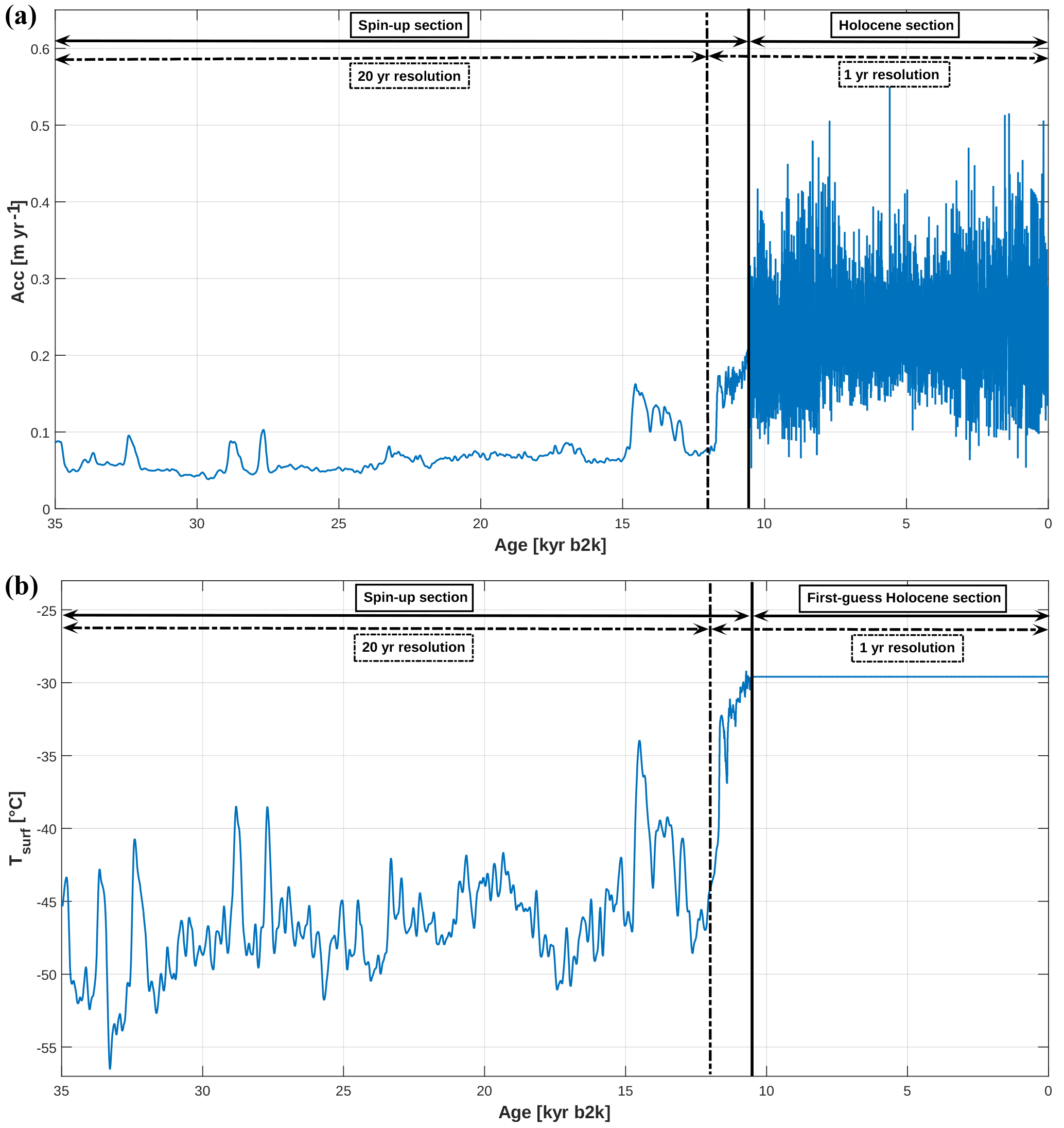
Figure 2(a) Used accumulation-rate input time series divided in a Holocene and a spin-up section, with time resolution in the Holocene section (20 to 10 520 years b2k) of 1 year. The time resolution for the transition between the Holocene and the spin-up section (10 520 to 12 000 years b2k) is 1 year as well. This is in opposition to the rest of the spin-up section which has a time resolution of 20 years. (b) Surface-temperature spin-up calculated from δ18Oice calibration. Time resolution equals the accumulation-rate spin-up section. The first-guess surface temperature input is simply a constant value.
2.1.1 Step 1: prior input
The starting point of the optimization procedure is the first guess. To construct the first-guess temperature input Tg,0(t), a constant temperature of −29.6 ∘C is used for the complete Holocene section, which corresponds to the last value of the temperature spin-up (Fig. 2b).
2.1.2 Step 2: Monte Carlo type input generator – generating long-term solutions
During the second step of the optimization, the prior temperature input Tg,0(t) from step 1 is iteratively (j) changed following a Monte Carlo approach. The basic idea of the Monte Carlo approach is to generate smooth temperature inputs Tmc,j(t) by superimposing low-pass-filtered values Pj of uniformly distributed random values Pr,j on the prior input . Then, the new input is fed to the firn model and the mismatch (with X≡δ15Nmc,j) between the modelled δ15Nmc,j (here Xmod), calculated from the model output, and the synthetic δ15Nsyn (here Xtarget) is computed for every time step (i) of the target data δ15Nsyn according to
(Note: if not otherwise stated, all mismatches in this study labelled with “D” are calculated similar to Eq. 1.)
Table 2Summary for the Monte Carlo approach: mismatch Dg,0 between the modelled δ15N (or temperature) values using the first-guess input and the synthetic δ15N (or temperature) target for each scenario. Dmc is the mismatch between the modelled δ15N (or temperature) using the final Monte Carlo temperature solution and the synthetic δ15N (or temperature) target for each scenario.
serves as the criterion which is minimized during the optimization in step 2. If the mismatch decreases compared to the prior input (, ), the new input is saved and used as the new guess (). This procedure is repeated until convergence is achieved, leading to the final long-term temperature Tmc,fin(t). Table 2 lists the number of improvements and iterations performed for the different synthetic datasets.
The perturbation of the current guess Tg,j is conducted in the following way: let be the vector containing the prior temperature input. A second vector (Pr,1) with the same number of elements nmc as Tg,0 is generated, containing nmc uniformly distributed random numbers within the limits of an also randomly (equally distributed) chosen standard deviation (SD). SD is chosen from a range of 0.05–0.50, which means that the maximum allowed perturbation of a single temperature value T(t0) is in a range of ±5 to ±50 %. Creating the synthetic frequencies, Pr,1 is low-pass filtered using cubic-spline filtering (Enting, 1987) with an equally distributed random cut-off period (COP) in the range of 500 to 2000 years generating the vector P1. Hereby the low-pass filtering of Pr,1 reduces the amplitudes of the perturbation of Tg,0. The new surface temperature input Tmc,1 is calculated from P1 according to
The superscript “T” stands for transposed and is the n by 1 matrix of ones.
This approach provides a high potential for parallel computing. In this study, an eight-core computer was used, generating and running eight different inputs of Tmc simultaneously, minimizing the time to find an improved solution. For example, during the 706 iterations for scenario S2, about 5600 different inputs were created and tested, leading to 351 improvements (see Table 2). Since it is possible to find more than one improvement per iteration step due to the parallelization on eight CPUs, the solution giving the minimal misfit is chosen as new first-guess for the next iteration step. This leads to a decrease of the used improvements for the optimization (e.g. for S2, 172 of the 351 improvements were used). Additionally, a first gas-age scale (Δagemc,fin(t)) is extracted from the model using the last improved conditions, which will then be used in step 3.
2.1.3 Step 3: adding short-term (high-frequency) information
In step 3, the missing short-term temperature history providing a suitable fit between modelled and synthetic δ15N data is directly extracted from the pointwise mismatch , between the modelled δ15Nmc,fin(t) obtained in step 2 and the synthetic δ15Nsyn target. Note that for a real reconstruction, this mismatch is calculated using the measured δ15Nmeas dataset instead of the synthetic one. can be interpreted in first order as the detrended high-frequency signal of the synthetic δ15Nsyn target. is transferred to the gas-age scale using Δagemc,fin(t) provided by the firn-model output for the smooth temperature input Tmc,fin(t). This is needed to insure synchroneity between the high-frequency temperature variations ΔT(t) extracted from the mismatch on the ice-age scale and the smooth temperature solution Tmc,fin(t). Additionally, the signal is shifted by about 10 years towards modern values to account for gas diffusion from the surface to the lock-in depth (Schwander et al., 1993), which is not yet implemented in the firn model. This is necessary for adding the calculated short-term temperature changes ΔT(t) to the smooth signal Tmc,fin(t). The ΔT values are calculated according to Eq. (3):
using the thermal-diffusion sensitivity for nitrogen-isotope fractionation from Grachev and Severinghaus (2003):
is the mean firn temperature in Kelvin which is calculated by the firn model for each time point i. To reconstruct the final (high-frequency) temperature input (Thf(t)), the extracted short-term temperature signal ΔT(t) is simply added to the long-term temperature input Tmc,fin(t):
2.1.4 Step 4: final correction of the surface temperature solution
For a further improvement of the remaining δ15N and resulting surface-temperature misfits (, ), it is important to find a correction method that contains information that is also available when using measured data. The benefit of the synthetic data study is that several later-unknown quantities can be calculated and used for improving the reconstruction approach (see Sects. 3 and 4). For instance, it is possible to split the synthetic δ15Nsyn data in the gravitational and thermodiffusion parts or to use the temperature misfit, which is unknown in reality. The idea underlying the correction algorithm explained hereafter is that the remaining misfits of δ15N () and temperature () are connected to the Monte Carlo (step 2) and high-frequency part (step 3) of the reconstruction algorithm. In the present inversion framework, it is not possible to find a long-term solution δ15Nmc,fin (or Tmc,fin) which exactly passes through the δ15Nsyn (or Tsyn) target in the middle of the variance in all parts of the time series. This leads to a slight over- or underestimation of δ15Nmc,fin(t) and their corresponding temperature values Tmc,fin(t). For example, a slightly too low (or too high) smooth temperature estimate Tmc,fin leads to a small increase (or decrease) of the firn-column height, creating a wrong gravitational background signal in δ15Nmc,fin on a later point in time (because the firn column needs some time to react). An additional error in the thermal-diffusion signal is also created due to the high-frequency part of the reconstruction (step 3), because the high-frequency information is directly extracted from the deviation of the synthetic target δ15Nsyn(t) and the modelled δ15Nmc,fin(t) from the final long-term solution Tmc,fin(t) of the Monte Carlo part. Therefore, this error is transferred into the next step of the reconstruction and partly creates the remaining deviations.
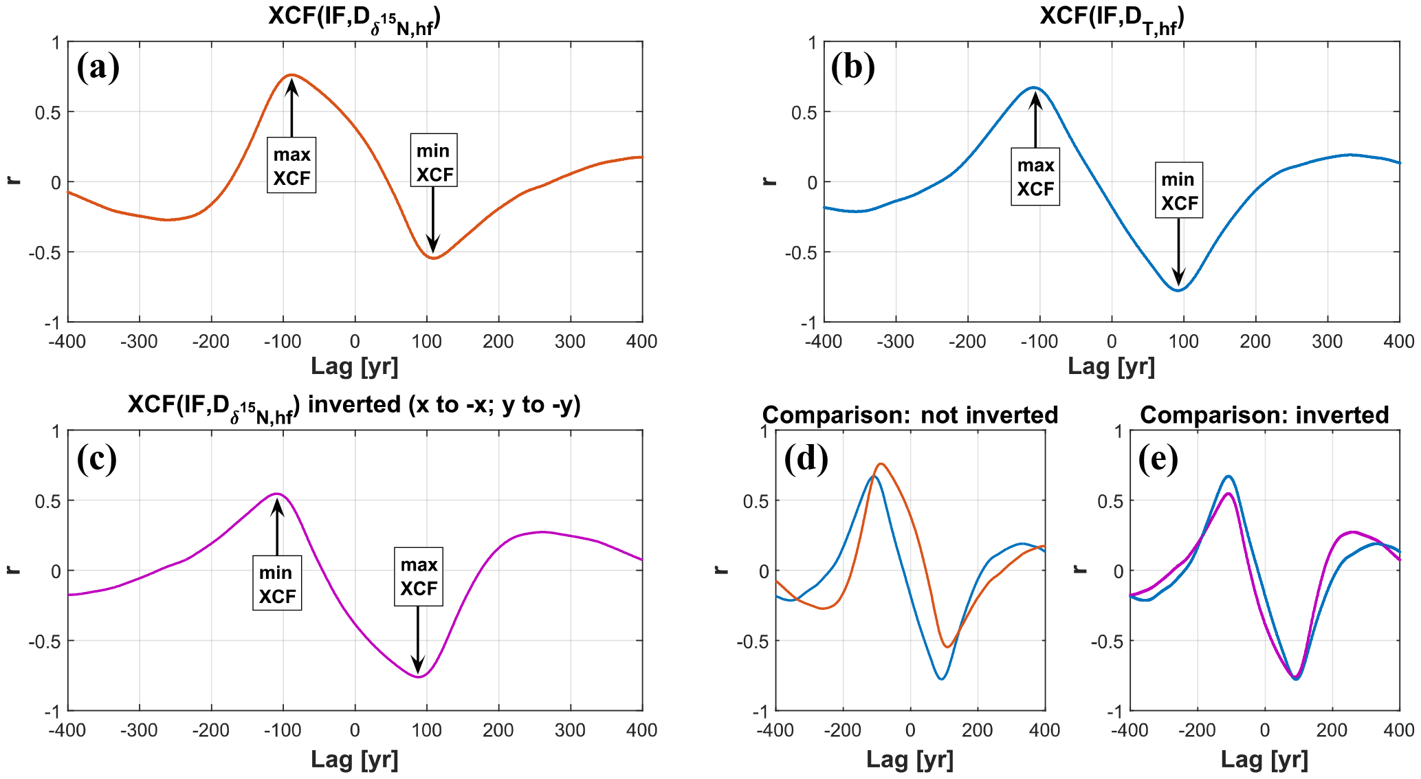
Figure 3Scenario S1: (a) cross-correlation function (xcf) between IF(t) and the remaining mismatch in δ15N (), after the high-frequency part shows two extrema: the maximum correlation (max xcf) and the minimum correlation (min xcf). (b) Cross-correlation function (xcf) between IF(t) and the remaining mismatch in temperature (), after the high-frequency part, shows two extrema: the maximum correlation (max xcf) and the minimum correlation (min xcf). (c) Inverting of panel (a) in x (lag) and y (correlation coefficient) direction. (d) Comparison between panels (a) and (b). (e) Comparison between panels (a) and (c). The temperature-correction values are calculated from the linear dependency between IF(t) and . After shifting IF(t) to max xcf (lag max) and to min xcf (lag min), Δδ15Nmax(t) and Δδ15Nmin(t) are calculated. Next, Δδ15Nmax(t) and Δδ15Nmin(t) are inverted. That means, for Δδ15Nmax(t), the values are shifted back (−lag max) and shifted further to lag min. After inverting, Δδ15Nmax(t) and Δδ15Nmin(t) are summed up component-wise to calculate Δδ15Ncv(t). Using Δδ15Ncv(t) in Eq. (3) leads to the temperature-correction values which are added to the temperature Thf.
To investigate this problem, the deviations of the synthetic target data δ15Nsyn to δ15Nmc,fin of the Monte Carlo part are numerically integrated over a time window of 200 years (Sect. 4, Supplement Sect. S3), and thereafter the window is shifted from past to future in 1-year steps resulting in a time series called IF(t). IF(t) equals a 200-year running mean of . For t, the middle position of the window is allocated. The time evolution of IF(t) is a measure for the deviation of the long-term solution δ15Nmc,fin(t) (or Tmc,fin(t)) from the perfect middle passage through the target data δ15Nsyn(t) (or Tsyn(t)) and for the slight over- and underestimation of the resulting temperature.
Next, the sample cross-correlation function (xcf) (Box et al., 1994) is applied to IF(t) and the remaining misfits of δ15N after the high-frequency part. The xcf shows two extrema (Fig. 3a), a maximum (xcfmax) and a minimum (xcfmin) at two certain lags (lag at xcf and lag at xcf). Now, the same analysis is conducted for IF(t) versus the temperature mismatch (Fig. 3b), which shows an equal behaviour (two extrema, lag at xcf and lag at xcf). Comparing the two cross correlations shows that lag equals the negative lag and lag corresponds to the negative lag (Fig. 3d, e). The idea for the correction is that the extrema in the cross-correlation IF(t) versus with the positive lag (positive means here that has to be shifted to past values relative to IF(t)) creates the misfit of temperature on the negative lag (modern direction) of IF(t) versus , and vice versa. So, IF(t) yields information about the cause and allows us to correct this effect between the remaining mismatches, and , over the whole time series. The lags are not sharp signals, due to the fact that (i) the cross correlations are conducted over the whole analysed record, leading to an averaging of this cause-and-effect relationship and that (ii) IF(t) is a smoothed quantity itself. The correction of the reconstructed temperature after the high-frequency part is conducted in the following way: from the two linear relationships between IF(t) and at the two lags (lag at xcf, lag at xcf), two sets of δ15N correction values (Δδ15Nmax(t) from xcf and Δδ15Nmin(t) from xcf) are calculated. Then, the lags are inverted (Fig. 3c, e), shifting the two sets of the δ15N correction values to the attributed lags of the cross correlation between IF(t) and (e.g. Δδ15Nmin(t) to lag from xcf from the cross correlation between IF(t) and ), therefore changing the time assignments of Δδ15Nmin(t) and Δδ15Nmax(t) to Δδ15N) and Δδ15N). Now, the Δδ15Nmax(t) and Δδ15Nmin(t) are summed up component-wise, leading to the time series Δδ15Ncv(t). From Eq. (3) with Δδ15Ncv,i instead of , the corresponding temperature correction values are calculated and added to the high-frequency temperature solution Thf(t), giving the corrected temperature Tcorr(t). Finally, Tcorr(t) is used to run the firn model to calculate the corrected δ15Ncorr(t) time series. This cause-and-effect relationship found in the cross correlations between IF(t) and , and IF(t) and , is exemplarily shown in Fig. 3 for scenario S1 and was found for all eight synthetic scenarios. The derived correction algorithm leads to a further reduction of the mismatches of about 40 % in δ15N and temperature (see Sect. 3.2).
2.2 Firn-densification and heat-diffusion model
Surface-temperature reconstruction relies on firn densification combined with gas and heat diffusion (Severinghaus et al., 1998). In this study, the firn-densification and heat-diffusion model, developed by Schwander et al. (1997), is used to reconstruct firn parameters for calculating synthetic δ15N values depending on the input time series. It is a semi-empirical model based on the work of Herron and Langway (1980) and Barnola et al. (1991), and implemented using the Crank and Nicholson algorithm (Crank, 1975), and was also used for the temperature reconstructions by Huber et al. (2006) and Kindler et al. (2014). Besides surface-temperature time series, accurate accumulation-rate data are needed to run the model. The model then calculates the densification and heat-diffusion history of the firn layer and provides parameters for calculating the fractionation of the nitrogen isotopes for each time step, according to the following equations:
δ15Ngrav(t) is the component of the isotopic fractionation due to the gravitational settling (Craig et al., 1988; Schwander, 1989) and depends on the lock-in depth (LID) zLID(t) and the mean firn temperature (Leuenberger et al., 1999). g is the gravitational acceleration, Δm the molar mass difference between the heavy and light isotopes (equal to 10−3 kg mol−1 for nitrogen) and R the ideal gas constant. zLID is defined as a density threshold ρLID, which is slightly sensitive to surface temperature, following the formula from Martinerie et al. (1994), with a small offset correction of 14 kg m−3 to account for the presence of a non-diffusive zone (Schwander et al., 1997):
where
The thermal-fractionation component of the δ15N signal (Severinghaus et al., 1998) is calculated using Eq. (8), where Tsurf(t) and Tbottom(t) stand for the temperatures at the top and the bottom of the diffusive firn layer. In contrast to Tsurf(t), which is an input parameter for the model, Tbottom(t) is calculated by the model for each time step. The thermal-diffusion constant αT was measured by Grachev and Severinghaus (2003) for nitrogen (Eq. 12):
The firn model used here behaves purely as a forward model, which means that for the given input time series the output parameters (here, finally δ15Nmod(t)) can be calculated, but it is not easily possible to construct from measured isotope data the related surface-temperature or accumulation-rate histories. The goal of the presented study is an automatization of this inverse-modelling procedure for the reconstruction of the rather small Holocene temperature variations.
2.3 Measurement, input data and timescale
2.3.1 Timescale
For the entire study, the GICC05 chronology is used (Rasmussen et al., 2014; Seierstad et al., 2014). During the whole reconstruction procedure, the two input time series (surface temperature and accumulation rate) are split into two parts. The first part ranges from 20 to 10 520 years b2k (called the “Holocene section”) and the second one from 10 520 to 35 000 years b2k (“spin-up section”). The entire accumulation-rate input, as well as the spin-up section of the surface-temperature input, remains unchanged during the reconstruction procedure.
2.3.2 Accumulation-rate data
Besides surface temperatures, accumulation-rate data are needed to drive the firn model. In this study, we use the original accumulation rates, reconstructed in Cuffey and Clow (1997), produced using an ice-flow model adapted to the Greenland Ice Sheet Project Two (GISP2) location but adapted to the GICC05 chronology (Rasmussen et al., 2008; Seierstad et al., 2014). A detailed description of the adaption procedure can be found in Sect. S1 of the Supplement. The raw accumulation-rate data for the main part of the spin-up section (12 000 to 35 000 years b2k) are linearly interpolated to a 20-year grid and low-pass filtered with a 200-year COP using cubic-spline filtering (Enting, 1987). For the Holocene section (20–10 520 years b2k) and the transition part between Holocene and spin-up section (10 520 to 12 000 years b2k), the raw accumulation-rate data are linearly interpolated to a 1-year grid to obtain equidistant integer point-to-point distances which are necessary for the reconstruction, and to preserve as much information as possible for this time period (Fig. 2a). Except for these technical adjustments, the accumulation-rate input remains unmodified, assuming high reliability of these data during the Holocene. The accumulation data were reconstructed using annual layer counting, and a thinning model which should lead to maximum relative uncertainty of 10 % for the first 1500 of the 3000 m ice core (Cuffey and Clow, 1997). From the three accumulation-rate scenarios reconstructed in Cuffey and Clow (1997) and adapted here to the GICC05 chronology, the intermediate one is chosen (red curves in Fig. S1 in the Supplement). Since the differences between the scenarios are not important for the evaluation of the reconstruction approach, they are not taken into account for this study.
Additionally, two sensitivity experiments were conducted (see Sect. S2 in the Supplement) in order to investigate (i) the influence of low-pass filtering of the high-resolution accumulation rates on the model outputs and (ii) the possible contribution of the accumulation-rate variability to the δ15N data during the Holocene. The first experiment shows that filtering the accumulation rates with cut-off periods in the range of 20 to 500 years has nearly no influence on the modelled δ15N or lock-in depth as long as the major trends are being conserved. The second experiment leads to the finding that the accumulation-rate variability explains about 12 to 30 % of δ15N variability. A total of 30 % corresponds to the 8.2 kyr event and 12 % to the mean of the whole Holocene period including the 8.2 kyr event. Hence, the influence of accumulation changes, excluding the extreme 8.2 kyr event, is generally below 10 % during most parts of the Holocene.
2.3.3 δ18Oice data
Oxygen-isotope data from the GISP2 ice-core-water samples measured at the University of Washington's Quaternary Isotope Laboratory are used to construct the surface-temperature input of the model spin-up (12 to 35 kyr b2k, Grootes et al., 1993; Grootes and Stuiver, 1997; Meese et al., 1994; Steig et al., 1994; Stuiver et al., 1995; data availability: Grootes and Stuiver, 1999). The raw δ18Oice data are filtered and interpolated in the same way as the accumulation-rate data for the spin-up part.
2.3.4 Surface-temperature spin-up
The surface-temperature history of the spin-up section (Fig. 2b) is obtained by calibrating the filtered and interpolated δ18Oice data (Eq. 13) using the values for the temperature sensitivity α18O and offset β found by Kindler et al. (2014) for the North Greenland Ice Core Project (NGRIP) ice core assuming a linear relationship of δ18Oice with temperature.
The values 35.2 ‰ and −31.4 ∘C are modern-time parameters for the GISP2 site (Grootes and Stuiver, 1997; Schwander et al., 1997). The spin-up is needed to bring the firn model to a well-defined starting condition that takes possible memory effects (influence of earlier conditions) of firn states into account.
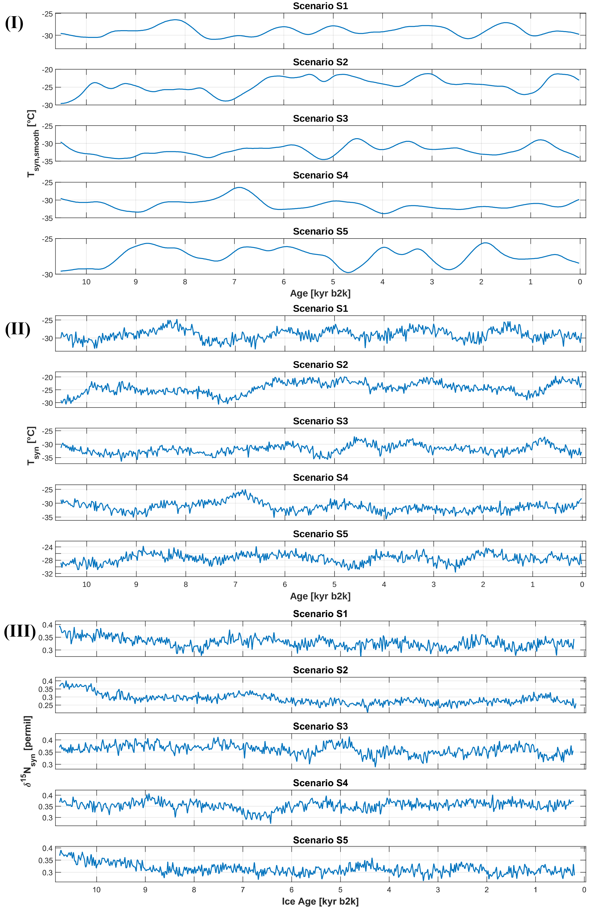
Figure 4(I) S1–S5: synthetic smooth temperature scenarios for the construction of the target-temperature data. (II) S1–S5: synthetic target surface-temperature scenarios. (III) S1–S5: corresponding synthetic δ15N target time series.
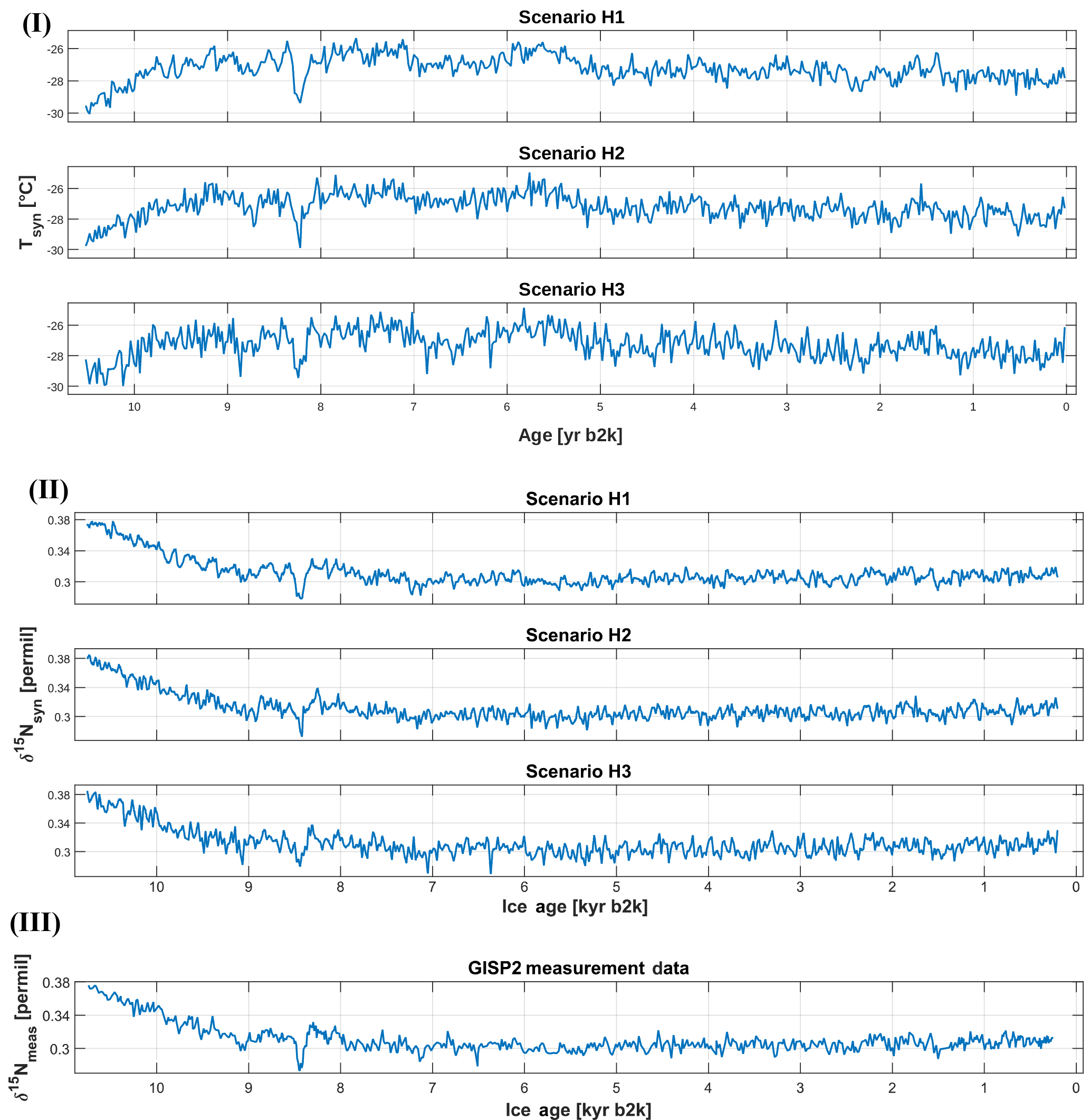
Figure 5(I) Synthetic target surface-temperature scenarios H1–H3. (II) Corresponding synthetic δ15N target time series H1–H3. (III) GISP2 δ15N measured data (Kobashi et al., 2008b).
2.3.5 Generating synthetic target data
In order to develop and evaluate the presented algorithm, eight temperature scenarios were constructed and used to model synthetic δ15N data, which serve later as targets for the reconstruction. From these eight synthetic surface-temperature and related δ15N scenarios (S1–S5 and H1–H3), three datasets (later called Holocene-like scenarios H1–H3) were constructed in such a way that the resulting δ15N time series are very close to the δ15N values measured by Kobashi et al. (2008b) in terms of variability (amplitudes) and frequency (data resolution) of the GISP2 nitrogen-isotope data (Figs. 4, 5).
The synthetic surface-temperature scenarios S1–S5 are created by generating a long-term temperature time series (Tsyn,smooth) analogous to the Monte Carlo part of the reconstruction procedure for only one iteration step (see Sect. 2.1). The values for the cut-off period used for the filtering of the random values, and the SD values (standard deviation of the random values; see Sect. 2.1) for the first five scenarios can be found in Table 3. The long-term temperatures (Fig. 4I) are calculated on a 20-year grid, which is nearly similar to the time resolution of the GISP2 δ15N measurement values of about 17 years (Kobashi et al., 2008b). For the Holocene-like scenarios, the smooth temperature time series were generated from the temperature reconstruction for the GISP2 δ15N data (not shown here). The final Holocene surface-temperature solution was filtered with a 100-year cut-off to obtain the long-term temperature scenario.
Following this, high-frequency information is added to the long-term temperature histories. A set of normally distributed random numbers with a zero mean and a standard deviation (1σ) of 1 K for scenarios S1–S5 and 0.3 K for Holocene-like scenarios H1–H3 is generated on the same 20-year grid and added up to the long-term temperature time series. Finally, the resulting synthetic target-temperature scenarios (Figs. 4II, 5I) are linearly interpolated to a 1-year grid.
Table 3Cut-off periods (COPs) and SD values used for creating the smooth synthetic temperature scenarios according to the Monte Carlo approach.
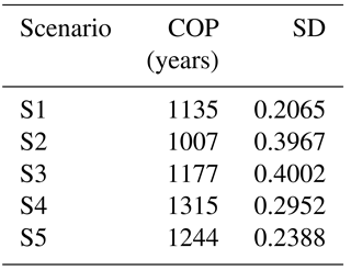
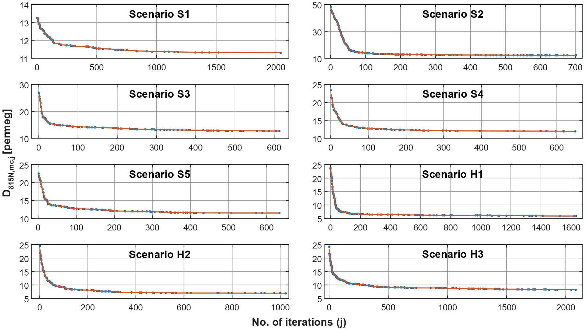
Figure 6Evolution of the mean misfit () of the modelled δ15Nmc versus synthetic target δ15Nsyn as function of the number of iterations (j) for the Monte Carlo approach for all synthetic target scenarios.
These synthetic temperatures are combined with the spin-up temperature and are used together with the accumulation-rate input to feed the firn model. From the model output, the synthetic δ15N targets are calculated according to Sect. 2.2. The firn-model output provides ice-age as well as gas-age information. The final synthetic δ15N target time series (δ15Nsyn) are set intentionally on the ice-age scale to mirror measured data, because no prior information is available for the gas-age – ice-age difference (Δage) for ice-core data.
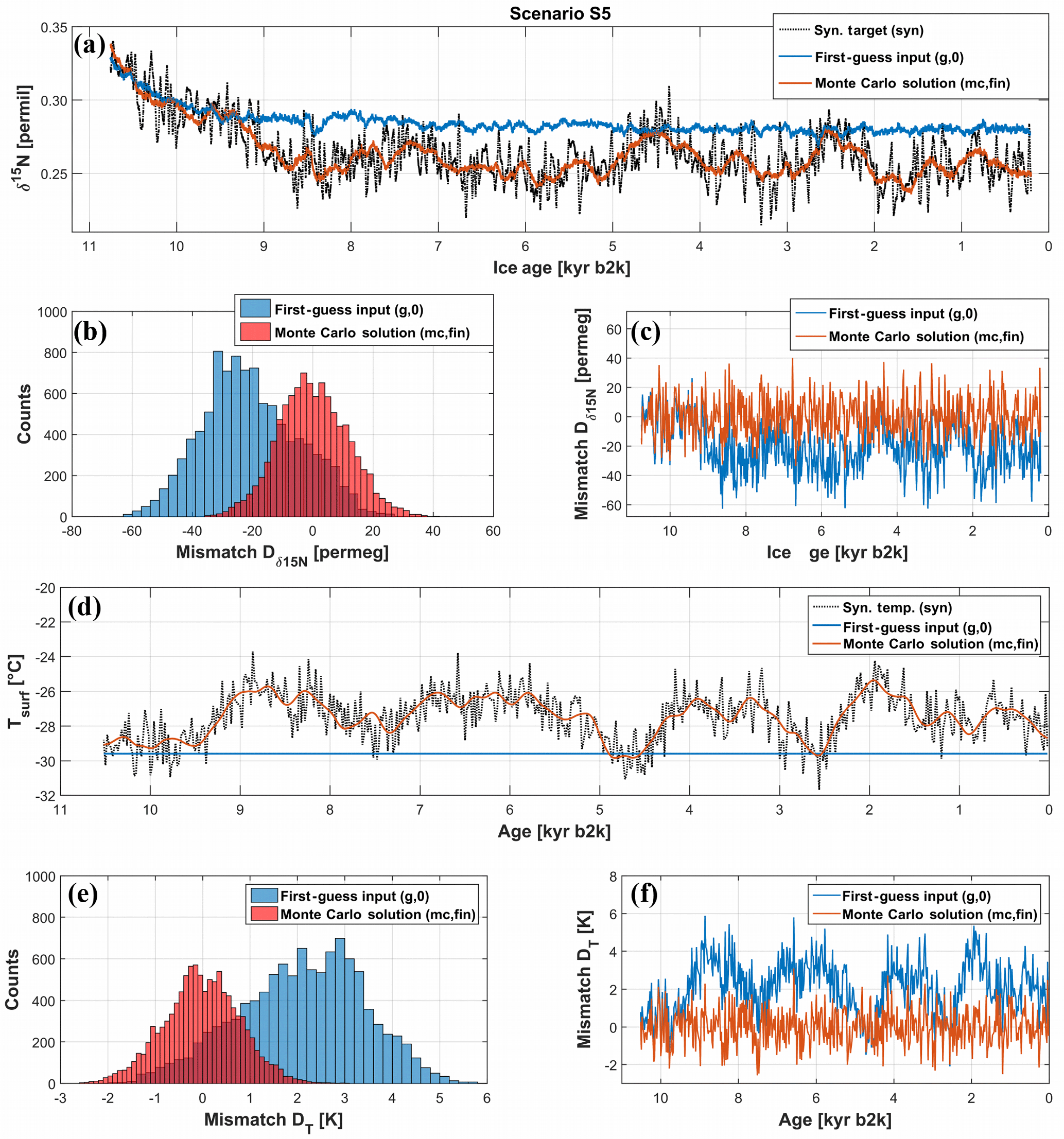
Figure 7(a–c) First-guess (g,0) versus Monte Carlo (mc,fin) δ15N solution for the scenario S5: (a) synthetic target δ15Nsyn (black dotted line), modelled δ15N time series for the first-guess input (blue line) and Monte Carlo solution (red line). (b) Histogram shows the pointwise mismatches of for the first-guess solution (blue) and the Monte Carlo solution (red) versus the synthetic target. (c) Time series of the pointwise mismatches of for the first-guess solution (blue) and the Monte Carlo solution (red) versus the synthetic target. (d–f) First-guess versus Monte Carlo surface-temperature solution Tsurf for the scenario S5: (d) synthetic surface-temperature target Tsyn (black dotted line), first-guess temperature input (blue line) and Monte Carlo solution (red line). (e) Histogram shows the pointwise temperature mismatches DTfor the first-guess solution (blue) and the Monte Carlo solution (red) versus the synthetic surface-temperature target. (f) Time series of the pointwise temperature mismatches DT for the first-guess solution (blue) and the Monte Carlo solution (red) versus the synthetic surface-temperature target.
3.1 Monte Carlo type input generator
Figure 6 shows the evolution of the misfit between the synthetic target data (δ15Nsyn) and the modelled output δ15Nmc,j of the Monte Carlo part (step 2) as a function of the applied iterations (j) for all synthetic scenarios. One can easily see that all scenarios show a steep decline of the mismatch during the first 50 to 200 iterations followed by a rather moderate decrease, which finally leads to a constant value. During the Monte Carlo part, it was possible to reduce the misfit compared to the first-guess solution by about 15 to 75 % depending on the scenario and the mismatch of the first-guess solution (see Table 2). This leads to a reduction of the temperature mismatches compared to the first-guess temperature mismatch of about 51 to 87 %.
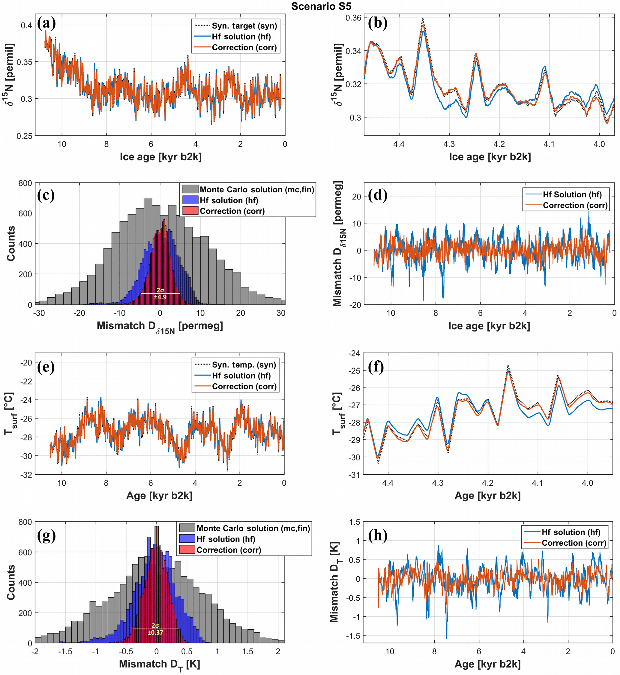
Figure 8(a–d) δ15N: (a) synthetic target δ15Nsyn (black dotted line), modelled δ15N time series after adding high-frequency information (hf, blue line) and correction (corr, red line) for the scenario S5. (b) Zoom-in for a randomly chosen 500-year interval shows the decrease of the mismatch after the correction compared to the high-frequency solution. (c) Histogram shows the pointwise mismatches of the synthetic target δ15Nsyn versus the Monte Carlo solution (mc,fin; grey), the high-frequency solution (hf; blue) and the correction (corr; red). The 95 % quantile is 4.9 permeg (yellow line) and used as an estimate for 2σ uncertainty of the final solution. (d) Time series of the pointwise mismatches of the synthetic target δ15Nsyn versus the high-frequency solution (hf; blue) and the correction (corr; red). (e–h) Temperature: (e) synthetic temperature target Tsyn (black dotted line), modelled temperature time series after adding high-frequency information (hf; blue line) and correction (corr; red line). (f) Zoom-in for a randomly chosen 500-year interval shows the decrease of the mismatch after the correction compared to the high-frequency solution. (g) Histogram shows the pointwise mismatches DT of the synthetic temperature target Tsyn versus the Monte Carlo solution (mc,fin; grey), the high-frequency solution (hf; blue) and the correction (corr; red). The 95 % quantile is 0.37 K (yellow line) and used as an estimate for 2σ uncertainty of the final solution. (h) Time series for the pointwise mismatches DT of the synthetic temperature target Tsyn versus the high-frequency solution (hf; blue) and the correction (corr; red).
Figure 7 provides the comparison between the first-guess (g,0; step 1) and Monte Carlo (mc,fin; step 2) solution versus the synthetic target data (syn) for the modelled δ15N (Fig. 7a–c) and surface-temperature values (Fig. 7d–f) for scenario S5. Subplots (a) and (d) show the time series of the synthetic target (black dotted line), the first-guess solution (blue line) and the Monte Carlo solution (red line) for δ15N and temperature. In subplots (b) and (e), the distribution of the pointwise mismatch Di of the first-guess (blue) and the Monte Carlo solutions (red) versus the synthetic target data for δ15N () and temperature (DT) can be found. Subplots (c) and (f) contain the time series for and . The data (red) are used to calculate the high-frequency signal that is superimposed to the long-term temperature solution Tmc,fin according to Eqs. (3) and (5) (see Sect. 2.1, step 3). From Fig. 7, it can be concluded that the Monte Carlo part of the reconstruction algorithm (step 2) leads to two major improvements of the first-guess solution. First, it is obvious that the Monte Carlo approach corrects the offsets of the first-guess input (g,0), which shifts the midpoint of the distributions of and to zero (see blue against red in Fig. 7b, e). The second improvement is that the distributions become more symmetric and the misfit is overall reduced (the distributions become narrower) compared to the first guess due to the middle passage through the δ15Nsyn targets. These improvements can be observed for all eight synthetic scenarios, showing the robustness of the Monte Carlo part (see Table 2, Fig. 7).
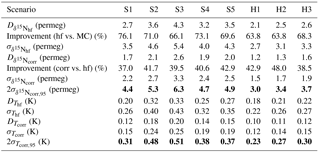
Table 4Summary for the high-frequency (hf) and correction part (corr) of the reconstruction approach. D is the mean mismatch between the modelled δ15N (or temperature) data and the synthetic δ15N (or temperature) target. σ is the standard deviation of the pointwise mismatches Di. The 95 % quantiles (2 or 2) of the pointwise δ15N (or temperature) mismatches are used as an estimate for the 2σ uncertainty for the final solution (values in bold).
3.2 High-frequency step and final correction
Figure 8 provides the comparison between the Monte Carlo (mc,fin; step 2), the high-frequency (hf; step 3) and the correction (corr; step 4) parts of the reconstruction procedure for the scenario S5. Additional data for all other scenarios can be found in Table 4. The upper four plots (Fig. 8a–d) illustrate each reconstruction step and their effect on the modelled δ15N; the bottom four plots (Fig. 8e–h) show the corresponding results on the temperature. Plots (a) and (e) contain the time series of the synthetic δ15Nsyn or Tsyn target (syn; black dotted line), the high-frequency solution (hf; blue line) and the final solution after the correction part (corr; red line). For visibility reasons, subplots (b) and (f) display a zoom-in for a randomly chosen time window of about 500 years for the same quantities, which shows the excellent agreement in timing and amplitudes of the modelled δ15N and temperature compared to the synthetic target data. Histograms (c) and (g) and subplots (d) and (h) show the distribution and the time series of the pointwise mismatches ( for δ15N; for temperature) between the modelled and the synthetic target data in δ15N and temperature for each reconstruction step.
Compared to the Monte Carlo solution, the high-frequency part leads to a large refinement of the reconstructions. For the mean δ15N misfits , the improvement between the Monte Carlo and the high-frequency parts is in the range of 64 to 76 % (see Table 4). This leads to a reduction of the temperature mismatches DT of 43 to 67 %. The standard deviations (1σ) of the pointwise mismatches (Fig. 8c, d, g, h) in δ15N and temperature after the high-frequency parts are in the range of about 2.7 to 5.4 permeg (one permeg equals 10−6) for δ15N and 0.22 to 0.40 K for the reconstructed temperatures depending on the scenario, which is clearly visible in the decreasing width of the histograms (Fig. 8c and g, blue against grey).
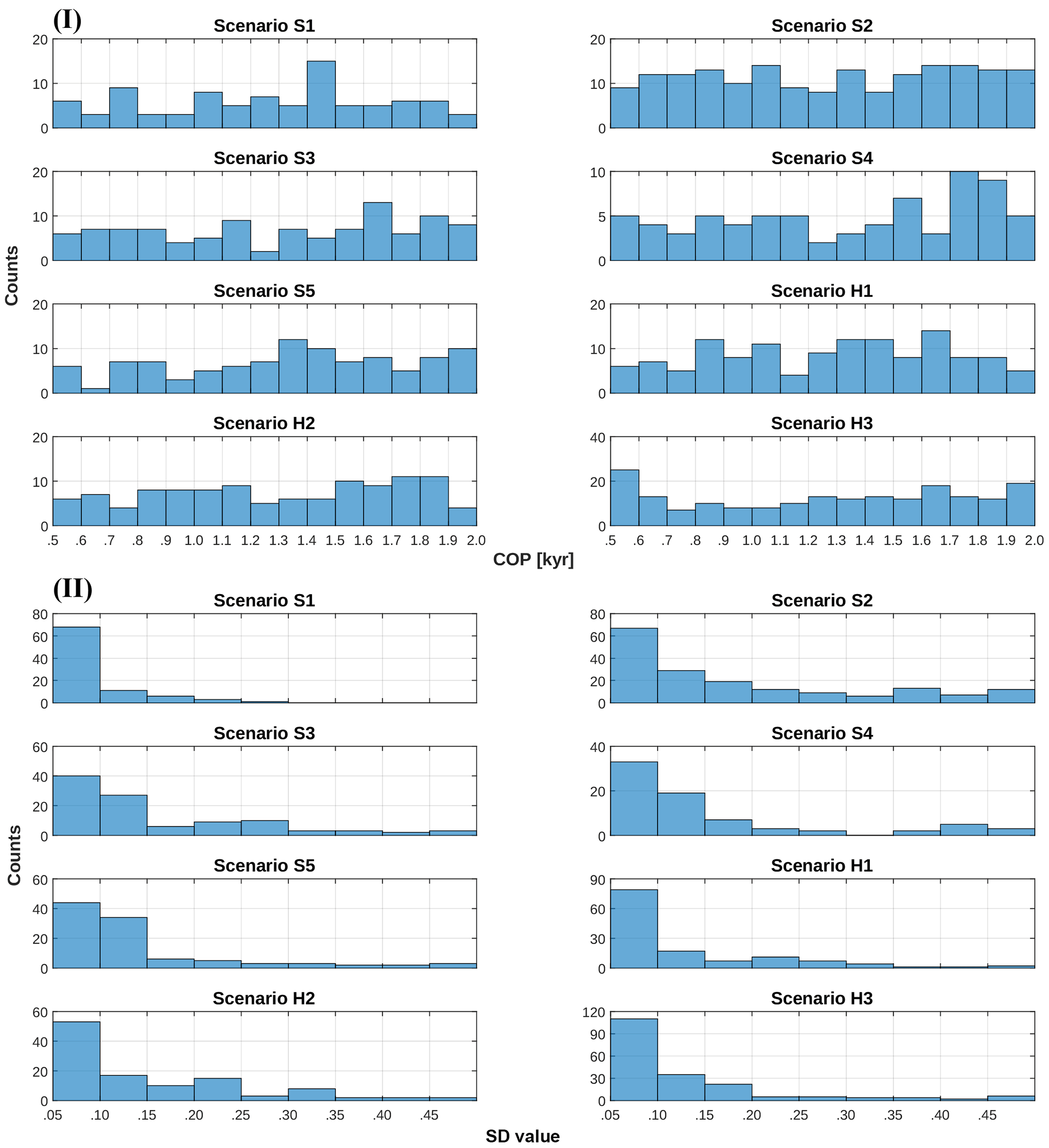
Figure 9(I) Counts of the COPs and (II) counts of the SD values used to create the improvements for the smooth temperature solutions of the Monte Carlo input generator for all synthetic scenarios (S1–S5 and H1–H3). A SD value of 0.1, for example, means that the maximum allowed perturbation of one temperature value T(t0) is ±10 %.
The mismatches after the correction part of the reconstruction approach show clearly a further decrease of the misfits. This means that the width of the distributions of the pointwise mismatches as well as is further reduced, and the distributions become more symmetric (long tales disappear; see histograms c and g; red against blue of Fig. 8). The time series of the mismatches (Fig. 8d and h) clearly illustrate that the correction approach mainly tackles the extreme deviations (sharp reduction of extreme values' occurrence in the red distribution compared to the blue distribution) leading to a further improvement of about 40 % in δ15N and temperature. Finally, the 95 % quantiles (2, 2) of the remaining pointwise mismatches of δ15N and temperature ( or ) were calculated for the final solutions for all scenarios and are used as an estimate for the 2σ uncertainty of the reconstruction algorithm (see Fig. 8c, g and Table 4). The final uncertainties (2σ) are of the order of 3.0 to 6.3 permeg for δ15N and 0.23 to 0.51 K for the surface temperature misfits. It is noteworthy that the measurement uncertainties (per point) of state-of-the-art δ15N measurements are of the same order of magnitude, i.e. 3 to 5 permeg (Kobashi et al., 2008b), highlighting the effectiveness of the presented fitting approach. Table 5 contains the final mismatches (2σ) in Δage between the synthetic target and the final modelled data after the correction step for all scenarios, and shows that with a known accumulation rate and assumed perfect firn physics, it is possible to fit the Δage history in the Holocene with mean uncertainties better than 2 years. In other words, the uncertainty in Δage reconstruction due to the inversion algorithm alone is of the order of 2 years.
4.1 Monte Carlo type input generator
Figure 9 shows the distribution of the COPs (I) and SD values (II) used to create the improvements (Sect. 2.1, step 2) for all scenarios. The cut-off periods are more or less evenly distributed, which shows that nearly all of the allowed frequency range (500 to 2000 years) was used to create the improvements during the iterations. In contrast, the distributions of the SD values show clearly that mostly small SD values are used to create the improvements, which implies that iterations with small perturbations will more likely lead to an improvement than larger ones.
Table 5Final mismatches Δ(Δage) (2σ) of Δage between the corrected solution and the synthetic targets for all scenarios.
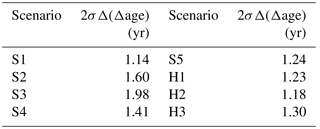
Figure 6 reveals a weak point of the Monte Carlo part, namely the absence of a suitable termination criterion for the optimization. The implementation until now is conducted such that the maximum number of iterations is given by the user or the iterations are terminated after a certain time (e.g. 15 h). Figure 6 shows that for nearly all scenarios it would be possible to stop the optimization after about 400 iterations, due to rather small additional improvements later on. This would decrease the time needed for the Monte Carlo part to about 10 h (a single iteration needs about 90 s). Since the goal of the Monte Carlo part is to find a temperature realization that leads to an optimal middle passage through the δ15N target data, it would be possible to use the mean difference between the δ15N target and spline-filtered δ15N data using a certain cut-off period as a termination criterion. This issue is under investigation at the moment. Another possibility to decrease the time needed for the Monte Carlo part could be an increase in the number of CPUs used for the parallelization of the model runs. For this study, an eight-core parallelization was used. A further increase in numbers of workers would improve the speed of the optimization.
4.2 High-frequency step and final correction
To investigate the timing and contributions of the remaining mismatches in δ15N and temperature for scenario S1 after the high-frequency (step 3) and correction parts (step 4), different cross-correlation experiments were conducted (see Sect. S3 in the Supplement). The experiments led to equal results. The major fraction of the final mismatches of δ15N emerges from mismatches in the thermal-diffusion component . Also a cancellation effect between the gravitational component and of the total mismatch in δ15N became obvious, affecting the calculation of lag and lag and most likely leading to a fundamental residual uncertainty in the low-permeg level for the corrected δ15N data. The same analyses were conducted for all synthetic scenarios, leading to similar results.
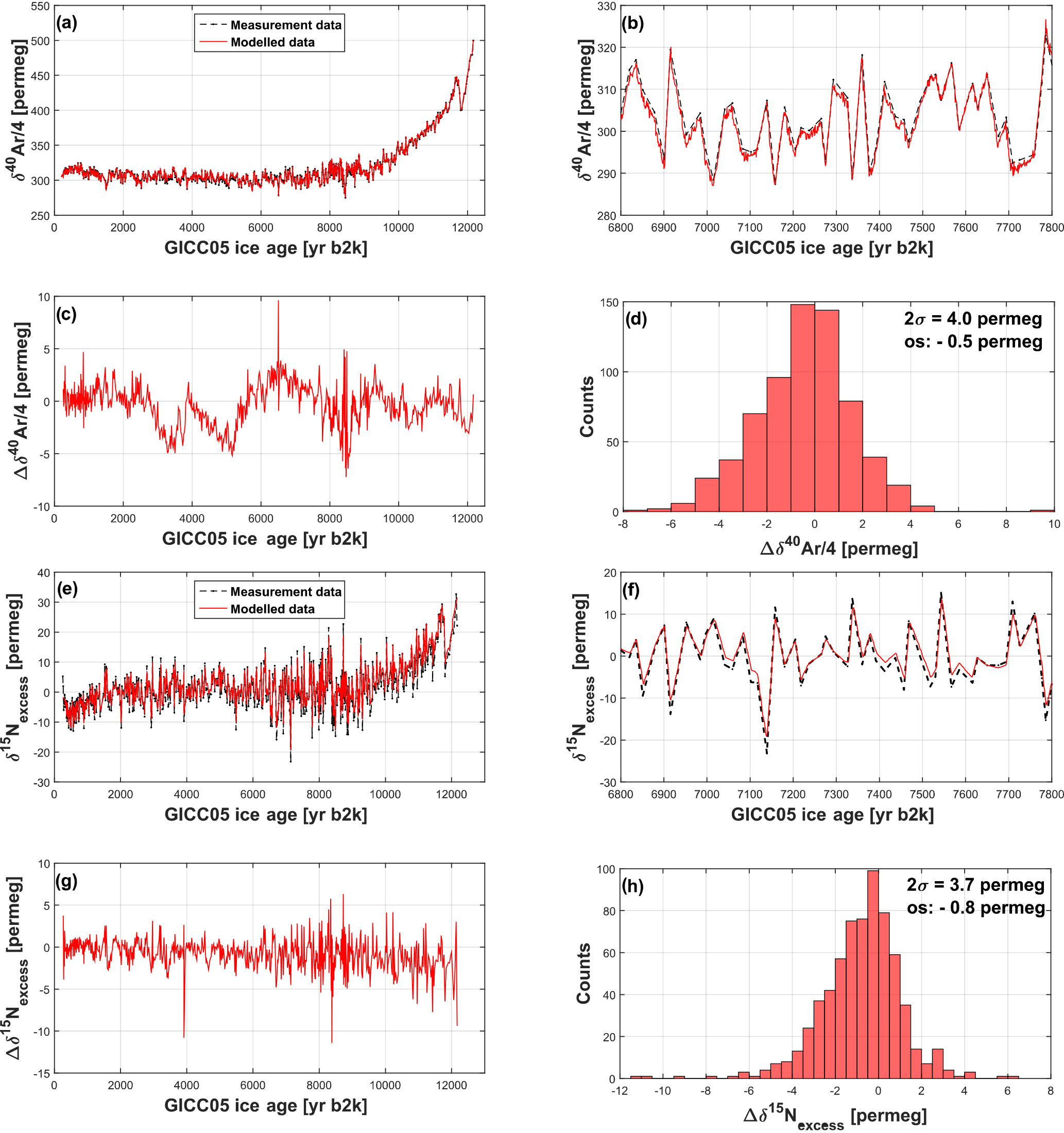
Figure 10Fitting of GISP2 Holocene δ40Ar (a–d) and δ15Nexcess (e–h) data (measurement data from Kobashi et al., 2008b): (a) measured versus modelled δ40Ar/4 time series. (b) Zoom-in for the same quantity as in panel (a). (c) Time series of the final mismatches Δδ40Ar/4 of the measured minus the modelled δ40Ar/4 data. (d) Histogram for the same quantity as in panel (c) showing an overall final mismatch (2σ) of 4.0 permeg and offset (os) of −0.5 permeg. (e) Measured versus modelled δ15Nexcess time series. (f) Zoom-in for the same quantity as in panel (e). (g) Time series of the final mismatches Δδ15Nexcess of the measured minus the modelled δ15Nexcess data. (h) Histogram for the same quantity as in panel (g) showing an overall final mismatch (2σ) of 3.7 permeg and offset (os) of −0.8 permeg.
Additionally, the influence of the window length, used for the calculation of IF(t), on the correction was analysed, showing that for all investigated window lengths the correction reduces the mismatches of δ15N and temperature, whatever correction mode was used (calculated with xcfmax, xcfmin or both quantities). Moreover, the correction is most efficient for window lengths in the range of 100 years to 300 years with an optimum at 200 years for all cases.
4.3 Key points to be considered for the application to real data
4.3.1 Benefits of the novel gas-isotope fitting approach
In addition to the fitting of δ15N data, the algorithm is able to fit δ40Ar and δ15Nexcess data as well using the same basic concepts (Fig. 10). Here, the δ40Ar and δ15Nexcess data from Kobashi et al. (2008b) were used as the fitting targets. We reach final mismatches (2σ) of 4.0 permeg for δ40Ar/4 and 3.7 permeg for δ15Nexcess, which are for both quantities below the analytical measurement uncertainty of 4.0 to 9.0 permeg for δ40Ar/4 and 5.0 to 9.8 permeg for δ15Nexcess measured data (Kobashi et al., 2008b).
The automated inversion of different gas-isotope quantities (δ15N, δ40Ar, δ15Nexcess) provides a unique opportunity to study the differences in the gained solutions using different targets and to improve our knowledge about the uncertainties of gas-isotope-based temperature reconstructions using a single firn model. Next, the presented algorithm is not dependent on the firn model, which leads to the implication that the algorithm can be coupled to different firn models describing firn physics in different ways. Furthermore, an automated reconstruction algorithm avoiding manual manipulation and leading to reproducible solutions makes it possible for the first time, to study and learn from the differences between solutions matching different targets. Finally, differences obtained by applying different firn physics (densification equations, convective zone, etc.) but the very same inversion algorithm may help to assess firn-model shortcomings, resulting in more robust uncertainty estimates than it was ever possible before.
In this publication, we show the functionality and the basic concepts of the automated inversion algorithm using well-known synthetic δ15N fitting targets. In this “perfect-world scenario”, the forward problem, converting surface temperature to δ15N, as well as the inverse problem, converting δ15N to surface temperature, are completely described by the used firn model. Consequently, all sources of signal noise are ignored. For the later use of the algorithm on δ15N, δ40Ar or δ15Nexcess measured data, this will not be the case anymore due to different sources of signal noise in the used measured data. As a result, differences between temperature solutions obtained from individual targets (δ15N, δ40Ar, δ15Nexcess) will become obvious. These differences will allow us to quantify the uncertainties associated with different unconstrained processes. Next, we will list and discuss potential sources of uncertainties and try to provide suggestions for their handling and quantification in our approach.
4.3.2 Measurement uncertainty and firn heterogeneity (centimetre-scale variability)
Many studies have investigated the influence of firn heterogeneity (or density fluctuations) on measurements of air compounds and quantities (e.g. δ15N, δ40Ar, CH4, CO2, O2 ∕ N2 ratio, air content) extracted from ice cores resulting in centimetre-scale variability and leading to additional noise on the measured data (e.g. Capron et al., 2010; Etheridge et al., 1992; Fourteau et al., 2017; Fujita et al., 2009; Hörhold et al., 2011; Huber and Leuenberger, 2004; Rhodes et al., 2013, 2016). Using discrete measurement techniques instead of continuous sampling methods makes it difficult to quantify these effects. However, during discrete analyses of ice-core air data, it is common to measure replicates for given depths, from which the measurement uncertainties of the gas-isotope data are calculated using pooled standard deviation (Hedges and Olkin, 1985). Often, it is not possible to take real replicates (same depth), and instead the replicates are taken from nearby depths. Hence, any potential centimetre-scale variability is to some degree already included in the measurement uncertainty, because each measurement point represents the average over a few centimetres of ice. This is especially the case for low-accumulation sites or glacial ice samples for which the vertical length of a sample (e.g. 10–25 cm long for the glacial part of the NGRIP ice core; Kindler et al., 2014) covers the equivalent of 20 to 50 years of ice at approximately 35 kyr b2k. Increasing the depth resolution of the samples would increase our knowledge of centimetre-scale variability, for, e.g. identifying anomalous entrapped gas layers that could have been rapidly isolated from the surface due to an overlying high-density layer (e.g. Rosen et al., 2014). As this variability is likely due to heterogeneity in the density profile, modelling such heterogeneities (if possible at all) may not help to better reconstruct a meaningful temperature history but rather to reproduce the source of noise. This means that the potential centimetre-scale variability, in many cases, is already incorporated in the analytical noise obtained from gas-isotope measurements, due to analytical techniques themselves. Assuming the measurement uncertainty as Gaussian distributed, it is easy to incorporate this source of uncertainty in the inverse-modelling approach presented here. This will increase the uncertainty of the temperature according to Eq. (3).The same equation can also be used for the calculation of the uncertainty in temperature related to measurement uncertainty in general.
To answer the pertinent question of how to better extract a meaningful temperature history from a noisy ice-core record, an excellent – but costly – solution is of course to use multiple ice cores. For example, a δ15N-based temperature reconstruction from the combination of data from the GISP2 ice core with the “sister ice core” GRIP drilled 30 km apart is likely one of the best ways to overcome potential centimetre-scale variability. A comparison of ice cores that were drilled even closer might be even more advantageous.
4.3.3 Smoothing effects due to gas diffusion and trapping
It is known that gas-diffusion and trapping processes in the firn can smooth out fast signals and result in a damping of the amplitudes of gas-isotope signals (e.g. Grachev and Severinghaus, 2005; Spahni, 2003). The duration of gas diffusion from the top of the diffusive column to the bottom where the air is closed off in bubbles is for Holocene conditions in Greenland approximately of the order of 10 years (Schwander et al., 1997), whereas the data resolution of the synthetic targets was set to 20 years to mimic the measurement data from Kobashi et al. (2008b) with a mean data resolution of about 17 years (see Sect. 2.3: “Generating synthetic target data”). In the study of Kindler et al. (2014), it was shown that a glacial Greenland lock-in depth leads to a damping of the δ15N signal of about 30 % for a 10 K temperature rise in 20 years. We further assume that the smoothing according to the lock-in process is negligible for Greenland Holocene conditions according to the much smaller amplitude signals and shallower LID. Yet, for glacial conditions, it requires attention.
4.3.4 Accumulation-rate uncertainties
For the synthetic data study presented in this paper, it is assumed that the used accumulation-rate data are well known with zero uncertainty. This simplification is used to show the functionality and basic concepts of the presented fitting algorithm in every detail on well-known δ15N and temperature targets and to focus on the final uncertainties originating from the presented fitting algorithm itself. For the later reconstruction using measured gas-isotope data together with the published accumulation-rate scenarios shown in Sect. S1 of the Supplement, this will not be the case anymore. Uncertainties in layer counting and corrections for ice thinning will lead to a fundamental uncertainty. Especially in the early Holocene, this can easily exceed 10 %. As the accumulation-rate data are used to run the firn model, all potential accumulation uncertainties are in part incorporated into the temperature reconstruction. On the other hand, as we discussed in Sect. S2 of the Supplement, the accumulation-rate variability has a minor impact compared to the input temperature on the variability of δ15N data in the Holocene. The influence of these quantities, accumulation rate or temperature, on the temperature reconstruction is not equal; during the Holocene, accumulation-rate variability explains about 12 to 30 % of δ15N variability. A total of 30 % corresponds to the 8.2 kyr event and 12 % to the mean of the whole Holocene period including the 8.2 kyr event. Hence, the influence of accumulation changes, excluding the extreme 8.2 kyr event, is generally below 10 % during the Holocene. If the accumulation is assumed to be completely correct, then the missing part will be assigned to temperature variations. Nevertheless, for the fitting of the Holocene measurement data, we will use all three accumulation-rate scenarios as shown in Sect. S1 of the Supplement. The difference in the reconstructed temperatures arising from the differences of these three scenarios will be used for the uncertainty calculation as well and is most likely higher than the uncertainty arising from uncertainties due to the process of producing the accumulation-rate data and from the conversion of the accumulation-rate data to the GICC05 timescale.
4.3.5 Convective zone variability
Many studies have shown the existence of a well-mixed zone at the top of the diffusive firn column, called the convective zone (CZ). The CZ is formed by strong katabatic winds and pressure gradients between the surface and the firn (e.g. Kawamura et al., 2006, 2013; Severinghaus et al., 2010). The existence of a CZ changes the gravitational background signal in δ15N and δ40Ar as it reduces the diffusive-column height. The presented fitting algorithm was used together with the two most frequently used firn models for temperature reconstructions based on stable isotopes of air, the Schwander et al. (1997) model which has no CZ built in (or better – a constant CZ of 0 m) and the Goujon firn model (Goujon et al., 2003) (which assumes a constant convective zone over time, that can easily be set in the code). This difference between the two firn models only changes significantly the absolute temperature rather than the temperature anomalies as it was shown by other studies (e.g. Guillevic et al., 2013, Fig. 3). In the presented work, we show the results using the model from Schwander et al. (1997), because the differences between the obtained solutions using the two models are negligible, except a constant temperature offset. Also noteworthy is that there is no firn model at the moment which uses a dynamically changing CZ. Indeed, this should be investigated but requires additional intense work. Additionally, the knowledge of the time evolution of CZ changes for time periods of millennia to several hundreds of millennia (in frequency and magnitude) is too poor to estimate the influence of this quantity on the reconstruction. In principle, it is possible to cancel out the influence of a potentially changing CZ by using δ15Nexcess data for temperature reconstruction, as due to the subtraction of δ40Ar/4 from δ15N the gravitational term of the signals is eliminated. From that point of view, it will be interesting to compare temperature solutions gained from δ15Nexcess fitting with the solutions based on δ15N or δ40Ar alone. This can offer a useful tool for quantifying the magnitude and frequency of CZ changes in the time interval of interest.
It is known that for some very low accumulation-rate sites in areas with strong katabatic winds (e.g. “megadunes”, Antarctica) extremely deep CZs can occur, which are potentially able to smooth out even decadal-scale temperature variations (Severinghaus et al., 2010). For this, its deepness would need to be of several dozens of metres, which is highly unrealistic even for glacial Summit conditions (Guillevic et al., 2013; see discussion in Annex A4, p. 1042) as well as for the rather stable Holocene period in Greenland for which no low accumulation and strong katabatic wind situations are to be expected.
4.4 Proof of concept for glacial data
For glacial conditions, the task of reconstructing temperature (with correct frequency and magnitude) without using δ18Oice information is much more challenging due to the highly variable gas-age – ice-age differences (Δage) between stadial and interstadial conditions. Here, contrary to the rather stable Holocene period, the Δage can vary by several hundreds of years. Also, the accumulation-rate data are more uncertain than for the Holocene. To prove that the presented fitting algorithm also works for glacial conditions, we inverted the δ15N data measured for the NGRIP ice core by Kindler et al. (2014) for two Dansgaard–Oeschger events, namely DO6 and DO7. Since the magnitudes of those events are higher and the signals are smoother than in the Holocene, we only had to use the Monte Carlo type input generator (see Sect. 2.1.2) for changing the temperature inputs. To compare our results to the δ18Oice-based and manually calibrated values from Kindler et al. (2014), we use the ss09sea06bm timescale (NGRIP members, 2004; Johnsen et al., 2001) as it was done in the Kindler et al. (2014) publication. For the model spin-up, we use the accumulation-rate and temperature data from Kindler et al. (2014) for the time span 36.2 to 60 kyr. The reconstruction window (containing DO6 and DO7) is set to 32 to 36.2 kyr. As the first-guess (starting point) of the reconstruction, we use the accumulation-rate data (Accg,0) for NGRIP from the ss09sea06bm timescale together with a constant temperature of about −49 ∘C for this time window. As minimization criterion Dg for the reconstruction, we simply use the sum of the root mean squared errors of the δ15N and Δage mismatches weighted with their uncertainties (wRMSE) according to the following equation, instead of the mean δ15N misfit alone as used for the Holocene (Eq. 1).
Here, and εΔage,k are the uncertainties in δ15N and Δage for the measured values i or k (Δage match points: Guillevic, 2013, p. 65, Table 3.2) and N, M the number of measurement values. We set permeg for all i (Kindler et al., 2014) and years for all k. The relative uncertainties in Δage can easily reach up to 50 % and more in the glacial period using the ss09sea06bm timescale which results in a pre-eminence of the δ15N misfits over the Δage misfits (10 to 20 % when using GICC05 timescale; Guillevic, 2013, p. 65 Table 3.2). Due to this issue, we have to set Δage uncertainties to 50 years to make both terms equally important for the fitting algorithm. In Fig. 11, we show preliminary results. The δ15N and Δage fitting (Fig. 11a, b) and the resulting gained temperature and accumulation-rate solutions (Fig. 11c, d) using the presented algorithm are completely independent from δ18Oice, which provides the opportunity to evaluate the δ18Oice-based reconstructions. In this study, the algorithm was used in three steps. First, starting with the first guess (constant temperature), the temperature was changed as explained before. The accumulation rate was changed in parallel to the temperature, allowing a random offset shift (up and down) together with a stretching or compressing (in y direction) of the accumulation-rate signal over the whole time window (32 to 36.2 kyr). This first step leads to the “Monte Carlo solution 0” (MCS0) which provides a first approximation and is the base for the next step. For the next step, we fixed the accumulation rate and let the algorithm only change the temperature to improve the δ15N fit (MCS1). Finally, we allow the algorithm to change the temperature together with the accumulation rate using the Monte Carlo type input generator for both quantities. This allows to change the shape of the accumulation-rate data. This final step can be seen as a fine tuning of the gained solutions from the steps before. The obtained mismatches in δ15N and Δage of all steps are at least of the same quality or better than the δ18Oice-based manual method from Kindler et al. (2014) (see Table 6). The gained temperature solutions show a very good agreement in timing and magnitude compared to the reconstruction of Kindler et al. (2014). Also, the accumulation-rate solutions show that the accumulation has to be reduced significantly compared to the ss09sea06bm data to allow a suitable fit of the δ15N and Δage target data, a result highly similar to Guillevic et al. (2013) and Kindler et al. (2014). The mismatches in δ15N and Δage of the final (MCS FIN) solution show a 15 % smaller misfit of δ15N (2σ) and an about 31 % smaller misfit of Δage (2σ) compared to the Kindler et al. (2014) solution. Keeping in mind that the used approach is completely independent from δ18Oice strengthens the functionality and quality of the presented gas-isotope fitting approach also for glacial reconstructions. As this section contains a proof of concept of the presented automated gas-isotope fitting algorithm on glacial data, preliminary results and ongoing work were shown here. Furthermore, as the presented fitting algorithm was developed and tested in first order for Holocene-like data, it is highly probable that the functionality of the algorithm using glacial data will be further extended and adjusted in future studies.
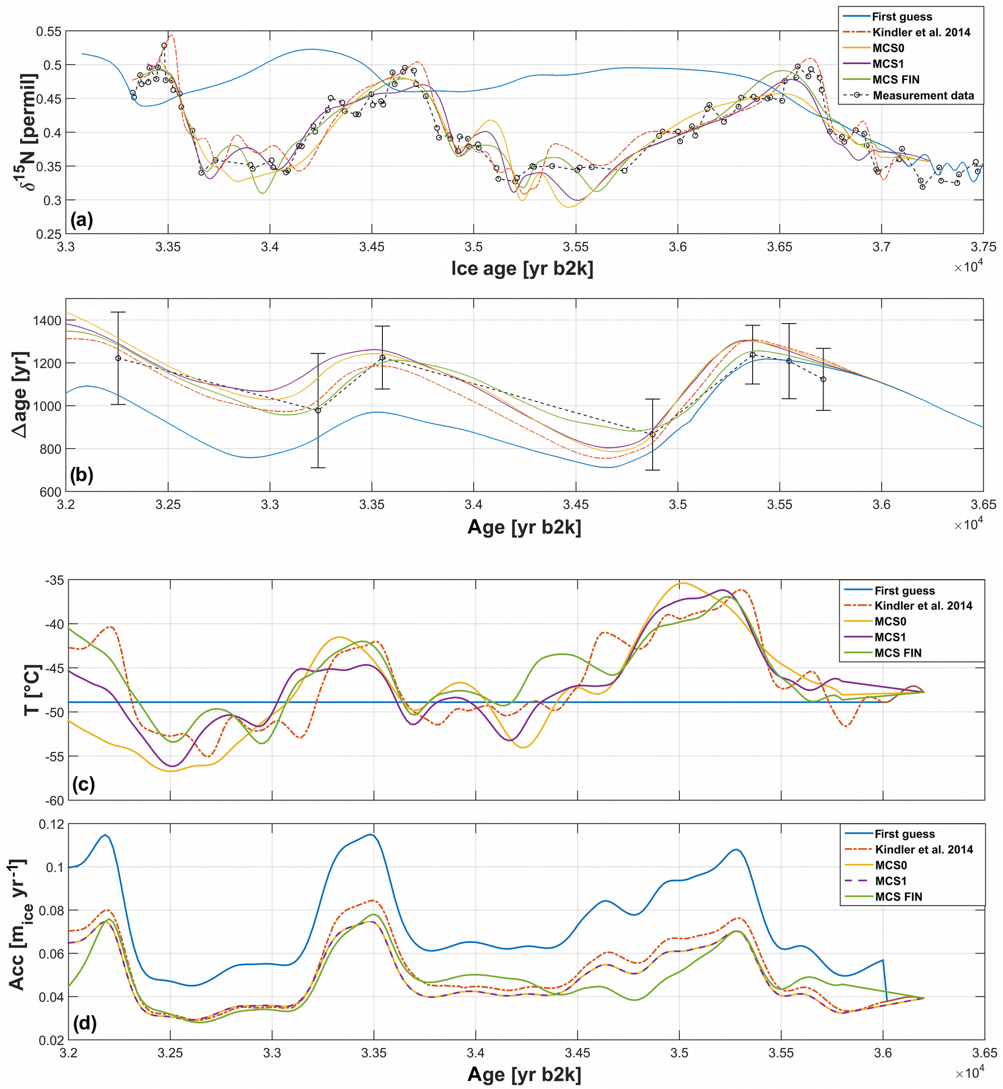
Figure 11Proof of concept for glacial reconstructions (NGRIP DO6 and DO7): (a) δ15N target plot: δ15N model output for the first-guess input (blue line), Kindler et al. (2014) fit (orange dotted line), Monte Carlo solution 0 (MCS0, yellow line), Monte Carlo solution 1 (MCS1, purple line), final Monte Carlo solution (MCS FIN, green line) and δ15N measurement target (black dotted line, measurement points are black cycles, data from Kindler et al., 2014). (b) Δage target plot: Δage model output for the first-guess input (blue line), Kindler et al. (2014) fit (orange dotted line), Monte Carlo solution 0 (MCS0, yellow line), Monte Carlo solution 1 (MCS1, purple line), final Monte Carlo solution (MCS FIN, green line) and Δage measurement target (black dotted line, measurement points are black cycles, data from Guillevic, 2013). (c) Temperature solution plot: first-guess input (blue line), Kindler et al. (2014) solution (orange dotted line), Monte Carlo solution 0 (MCS0, yellow line), Monte Carlo solution 1 (MCS1, purple line) and final Monte Carlo solution (MCS FIN, green line). (d) Accumulation-rate solution plot: first-guess input (blue line), Kindler et al. (2014) solution (orange dotted line), Monte Carlo solution 0 (MCS0, yellow line), Monte Carlo solution 1 (MCS1, purple line) and final Monte Carlo solution (MCS FIN, green line).
Table 6Proof of concept for glacial reconstruction: Dgl is the used minimization criterion (see Sect. 4.4).
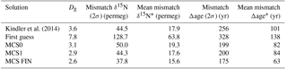
∗ The mean mismatches for δ15N and Δage were calculated according to Eq. (1).
A novel approach is introduced and described for inverting a firn-densification and heat-diffusion model to fit small gas-isotope-data variations as observed throughout the Holocene. From this new fitting method, it is possible to extract the surface-temperature history that drives the firn status which in turn leads to the gas-isotope time series. The approach is a combination of a Monte Carlo based iterative method and the analysis of remaining mismatches between modelled and target data. The procedure is fully automated and provides a high potential for parallel computing for time consumption optimization. Additional sensitivity experiments have shown that accumulation-rate changes have only a minor influence on short-term variations of δ15N, which themselves are mainly driven by high-frequency temperature variations. To evaluate the performances of the presented approach, eight different synthetic δ15N time series were created from eight known temperature histories. The fitting approach leads to an excellent agreement in timing and amplitudes between the modelled and synthetic δ15N and temperature data. The obtained final mismatches follow a symmetric standard-distribution function. A total of 95 % of the mismatches compared to the synthetic data are in an envelope between 3.0 to 6.3 permeg for δ15N and 0.23 to 0.51 K for temperature, depending on the synthetic temperature scenarios. These values can therefore be used as a 2σ estimate for the reconstruction uncertainty arising from the presented fitting algorithm itself. For δ15N, the obtained final uncertainties are of the same order of magnitude as state-of-the-art measurement uncertainty. The presented reconstruction approach was also successfully applied to δ40Ar and δ15Nexcess measured data. Moreover, we have shown that the presented fitting approach can also be applied to glacial temperature reconstructions with minor algorithm modifications. Based on the demonstrated flexibility of our inversion methodology, it is reasonable to adapt this approach for reconstructions of other non-linear physical processes.
The synthetic δ15N and temperature targets, the reconstructed δ15N and temperature data (using the synthetic δ15N as fitting targets), and the used accumulation rates can be found in the data supplement of this paper available at https://doi.pangaea.de/10.1594/PANGAEA.888997 (Döring and Leuenberger, 2018). The GISP2 δ18Oice data used in this study for calculating the temperature spin-up can be found in Grootes and Stuiver (1999). The source code for the inversion algorithm and additional auxiliary data are available upon request.
The supplement related to this article is available online at: https://doi.org/10.5194/cp-14-763-2018-supplement.
The authors declare that they have no conflict of interest.
This article is part of the special issue “Global Challenges for our Common Future: a paleoscience perspective” – PAGES Young Scientists Meeting 2017. It is a result of the 3rd Young Scientists Meeting (YSM), Morillo de Tou, Spain, 7–9 May 2017.
This work was supported by SNF grants (SNF-159563 and SNF-172550). We
would like to thank Takuro Kobashi, Philippe Kindler and Myriam Guillevic
for helpful discussions about the ice-core data and model
peculiarities.
Edited by: Emily Dearing Crampton Flood
Reviewed by: three anonymous referees
Barnola, J.-M., Pimienta, P., Raynaud, D., and Korotkevich, Y. S.: CO2-climate relationship as deduced from the Vostok ice core: a re-examination based on new measurements and on a re-evaluation of the air dating, Tellus B, 43, 83–90, https://doi.org/10.1034/j.1600-0889.1991.t01-1-00002.x, 1991.
Box, G. E. P., Jenkins, G. M., and Reinsel, G. C.: Time Series Analysis – Forecasting and Control, 3rd Edition, Prentice Hall, Englewood Cliff, New Jersey, USA, 1994.
Capron, E., Landais, A., Chappellaz, J., Schilt, A., Buiron, D., Dahl-Jensen, D., Johnsen, S. J., Jouzel, J., Lemieux-Dudon, B., Loulergue, L., Leuenberger, M., Masson-Delmotte, V., Meyer, H., Oerter, H., and Stenni, B.: Millennial and sub-millennial scale climatic variations recorded in polar ice cores over the last glacial period, Clim. Past, 6, 345–365, https://doi.org/10.5194/cp-6-345-2010, 2010.
Craig, H., Horibe, Y. and Sowers, T.: Gravitational separation of gases and isotopes in polar ice caps, Science, 242, 1675–8, https://doi.org/10.1126/science.242.4886.1675, 1988.
Crank, J.: The Mathematics of Diffusion, Clarendon, Oxford, UK, 414 pp., 1975.
Crausbay, S. D., Higuera, P. E., Sprugel, D. G., and Brubaker, L. B.: Fire catalyzed rapid ecological change in lowland coniferous forests of the Pacific Northwest over the past 14 000 years, Ecology, 98, 2356–2369, https://doi.org/10.1002/ecy.1897, 2017.
Cuffey, K. M. and Clow, G. D.: Temperature, accumulation, and ice sheet elevation in central Greenland through the last deglacial transition, J. Geophys. Res.-Oceans, 102, 26383–26396, https://doi.org/10.1029/96JC03981, 1997.
Cuffey, K. M., Clow, G. D., Alley, R. B., Stuiver, M., Waddington, E. D., and Saltus, R. W.: Large Arctic Temperature Change at the Wisconsin-Holocene Glacial Transition, Science, 270, 455–458, https://doi.org/10.1126/science.270.5235.455, 1995.
Dahl-Jensen, D., Mosegaard, K., Gundestrup, N., Clow, G. D., Johnsen, S. J., Hansen, A. W., and Balling, N.: Past Temperatures Directly from the Greenland Ice Sheet, Science, 282, 268–271, https://doi.org/10.1126/science.282.5387.268, 1998.
Dansgaard, W., Clausen, H. B., Gundestrup, N., Hammer, C. U., Johnsen, S. F., Kristinsdottir, P. M., and Reeh, N.: A new greenland deep ice core, Science, 218, 1273–7, https://doi.org/10.1126/science.218.4579.1273, 1982.
de Beaulieu, J. L., Brugiapaglia, E., Joannin, S., Guiter, F., Zanchetta, G., Wulf, S., Peyron, O., Bernardo, L., Didier, J., Stock, A., Rius, D., and Magny, M.: Lateglacial-Holocene abrupt vegetation changes at Lago Trifoglietti in Calabria, Southern Italy: The setting of ecosystems in a refugial zone, Quaternary Sci. Rev., 158, 44–57, https://doi.org/10.1016/j.quascirev.2016.12.013, 2017.
Denton, G. H. and Karlén, W.: Holocene climatic variations: their pattern and possible cause, Quaternary Res., 3, 155–205, https://doi.org/10.1016/0033-5894(73)90040-9, 1973.
Döring, M. and Leuenberger, M. C.: Synthetic and fitted d15N and temperature data and GISP2 accumulation rates (13.5–52 497.5 yr b2k) on GICC05 time scale, PANGAEA, https://doi.org/10.1594/PANGAEA.888997, 2018.
Enting, I. G.: On the Use of Smoothing Splines to Filter CO2 Data, J. Geophys. Res., 92, 10977–10984, https://doi.org/10.1029/JD092iD09p10977, 1987.
Etheridge, D. M., Pearman, G. I., and Fraser, P. J.: Changes in tropospheric methane between 1841 and 1978 from a high accumulation-rate Antarctic ice core, Tellus B, 44, 282–294, https://doi.org/10.1034/j.1600-0889.1992.t01-3-00006.x, 1992.
Fourteau, K., Faïn, X., Martinerie, P., Landais, A., Ekaykin, A. A., Lipenkov, V. Ya., and Chappellaz, J.: Analytical constraints on layered gas trapping and smoothing of atmospheric variability in ice under low-accumulation conditions, Clim. Past, 13, 1815-1830, https://doi.org/10.5194/cp-13-1815-2017, 2017.
Fujita, S., Okuyama, J., Hori, A., and Hondoh, T.: Metamorphism of stratified firn at Dome Fuji, Antarctica: A mechanism for local insolation modulation of gas transport conditions during bubble close off, J. Geophys. Res.-Sol. Ea., 114, F03023, https://doi.org/10.1029/2008JF001143, 2009.
Goujon, C., Barnola, J.-M., and Ritz, C.: Modeling the densification of polar firn including heat diffusion: Application to close-off characteristics and gas isotopic fractionation for Antarctica and Greenland sites, J. Geophys. Res.-Atmos., 108, 4792, https://doi.org/10.1029/2002JD003319, 2003.
Grachev, A. M. and Severinghaus, J. P.: Laboratory determination of thermal diffusion constants for 29N2/28N2 in air at temperatures from −60 to 0 ∘C for reconstruction of magnitudes of abrupt climate changes using the ice core fossil-air plaeothermometer, Geochim. Cosmochim. Ac., 67, 345–360, https://doi.org/10.1016/S0016-7037(02)01115-8, 2003.
Grachev, A. M. and Severinghaus, J. P.: A revised +10 ± 4 ∘C magnitude of the abrupt change in Greenland temperature at the Younger Dryas termination using published GISP2 gas isotope data and air thermal diffusion constants, Quaternary Sci. Rev., 24, 513–519, https://doi.org/10.1016/j.quascirev.2004.10.016, 2005.
Grootes, P. M. and Stuiver, M.: Oxygen 18/16 variability in Greenland snow and ice with 10−3- to 105-year time resolution, J. Geophys. Res.-Oceans, 102, 26455–26470, https://doi.org/10.1029/97JC00880, 1997.
Grootes, P. M. and Stuiver, M.: GISP2 Oxygen Isotope Data, PANGAEA, https://doi.org/10.1594/PANGAEA.56094, 1999.
Grootes, P. M., Stuiver, M., White, J. W. C., Johnsen, S., and Jouzel, J.: Comparison of oxygen isotope records from the GISP2 and GRIP Greenland ice cores, Nature, 366, 552–554, https://doi.org/10.1038/366552a0, 1993.
Guillevic, M.: Characterisation of rapid climate changes through isotope analyses of ice and entrapped air in the NEEM ice core, PhD thesis, University of Copenhagen, Copenhagen, Denmark, Université de Versailles Saint Quentin en Yvelines, Versailles, France, 2013.
Guillevic, M., Bazin, L., Landais, A., Kindler, P., Orsi, A., Masson-Delmotte, V., Blunier, T., Buchardt, S. L., Capron, E., Leuenberger, M., Martinerie, P., Prié, F., and Vinther, B. M.: Spatial gradients of temperature, accumulation and δ18O-ice in Greenland over a series of Dansgaard–Oeschger events, Clim. Past, 9, 1029–1051, https://doi.org/10.5194/cp-9-1029-2013, 2013.
Hedges, L. V. and Olkin, I.: Statistical methods for meta-analysis, Academic Press, San Diego, USA, 1985.
Herron, M. M. and Langway, C. C.: Firn densification: an empirical model, J. Glaciol., 25, 373–385, https://doi.org/10.1017/S0022143000015239, 1980.
Holmgren, K., Gogou, A., Izdebski, A., Luterbacher, J., Sicre, M. A., and Xoplaki, E.: Mediterranean Holocene climate, environment and human societies, Quaternary Sci. Rev., 136, 1–4, https://doi.org/10.1016/j.quascirev.2015.12.014, 2016.
Hörhold, M. W., Kipfstuhl, S., Wilhelms, F., Freitag, J., and Frenzel, A.: The densification of layered polar firn, J. Geophys. Res.-Earth, 116, F01001, https://doi.org/10.1029/2009JF001630, 2011.
Huber, C. and Leuenberger, M.: Measurements of isotope and elemental ratios of air from polar ice with a new on-line extraction method, Geochem. Geophy. Geosy., 5, Q10002, https://doi.org/10.1029/2004GC000766, 2004.
Huber, C., Leuenberger, M., Spahni, R., Flückiger, J., Schwander, J., Stocker, T. F., Johnsen, S., Landais, A., and Jouzel, J.: Isotope calibrated Greenland temperature record over Marine Isotope Stage 3 and its relation to CH4, Earth Planet. Sc. Lett., 243, 504–519, https://doi.org/10.1016/j.epsl.2006.01.002, 2006.
Johnsen, S. J., Clausen, H. B., Dansgaard, W., Fuhrer, K., Gundestrup, N., Hammer, C. U., Iversen, P., Jouzel, J., Stauffer, B., and Steffensen, J. P.: Irregular glacial interstadials recorded in a new Greenland ice core, Nature, 359, 311–313, https://doi.org/10.1038/359311a0, 1992.
Johnsen, S. J., Dahl-Jensen, D., Gundestrup, N., Steffensen, J. P., Clausen, H. B., Miller, H., Masson-Delmotte, V., Sveinbjörnsdottir, A. E., and White, J.: Oxygen isotope and palaeotemperature records from six Greenland ice-core stations: Camp Century, Dye-3, GRIP, GISP2, Renland and NorthGRIP, J. Quaternary Sci., 16, 299–307, https://doi.org/10.1002/jqs.622, 2001.
Kawamura, K., Severinghaus, J. P., Ishidoya, S., Sugawara, S., Hashida, G., Motoyama, H., Fujii, Y., Aoki, S., and Nakazawa, T.: Convective mixing of air in firn at four polar sites, Earth Planet. Sc. Lett., 244, 672–682, https://doi.org/10.1016/j.epsl.2006.02.017, 2006.
Kawamura, K., Severinghaus, J. P., Albert, M. R., Courville, Z. R., Fahnestock, M. A., Scambos, T., Shields, E., and Shuman, C. A.: Kinetic fractionation of gases by deep air convection in polar firn, Atmos. Chem. Phys., 13, 11141–11155, https://doi.org/10.5194/acp-13-11141-2013, 2013.
Kindler, P., Guillevic, M., Baumgartner, M., Schwander, J., Landais, A., and Leuenberger, M.: Temperature reconstruction from 10 to 120 kyr b2k from the NGRIP ice core, Clim. Past, 10, 887–902, https://doi.org/10.5194/cp-10-887-2014, 2014.
Kobashi, T., Severinghaus, J. P., and Barnola, J. M.: 4 ± 1.5 ∘C abrupt warming 11 270 yr ago identified from trapped air in Greenland ice, Earth Planet. Sc. Lett., 268, 397–407, https://doi.org/10.1016/j.epsl.2008.01.032, 2008a.
Kobashi, T., Severinghaus, J. P., and Kawamura, K.: Argon and nitrogen isotopes of trapped air in the GISP2 ice core during the Holocene epoch (0–11 500 B.P.): Methodology and implications for gas loss processes, Geochim. Cosmochim. Ac., 72, 4675–4686, https://doi.org/10.1016/j.gca.2008.07.006, 2008b.
Kobashi, T., Kawamura, K., Severinghaus, J. P., Barnola, J. M., Nakaegawa, T., Vinther, B. M., Johnsen, S. J., and Box, J. E.: High variability of Greenland surface temperature over the past 4000 years estimated from trapped air in an ice core, Geophys. Res. Lett., 38, L21501, https://doi.org/10.1029/2011GL049444, 2011.
Kobashi, T., Menviel, L., Jeltsch-Thömmes, A., Vinther, B. M., Box, J. E., Muscheler, R., Nakaegawa, T., Pfister, P. L., Döring, M., Leuenberger, M., Wanner, H., and Ohmura, A.: Volcanic influence on centennial to millennial Holocene Greenland temperature change, Sci. Rep., 7, 1441, https://doi.org/10.1038/s41598-017-01451-7, 2017.
Landais, A., Barnola, J. M., Masson-Delmotte, V., Jouzel, J., Chappellaz, J., Caillon, N., Huber, C., Leuenberger, M., and Johnsen, S. J.: A continuous record of temperature evolution over a sequence of Dansgaard-Oeschger events during Marine Isotopic Stage 4 (76 to 62 kyr BP), Geophys. Res. Lett., 31, 1–4, https://doi.org/10.1029/2004GL021193, 2004.
Lespez, L., Carozza, L., Berger, J.-F., Kuzucuoglu, C., Ghilardi, M., Carozza, J.-M., and Vanniere, B.: Rapid climatic change and social transformations Uncertainties, adaptability and resilience, in: The Mediterranean Region under Climate Change, A Scientific Update, edited by: Thiébault, S. and Moatti J.-P., IRD Éditions, Institut De Recherche Pour Le Développement, Marseille, France, 35–45, 2016.
Leuenberger, M. C., Lang, C., and Schwander, J.: Delta15N measurements as a calibration tool for the paleothermometer and gas-ice age differences: A case study for the 8200 B.P. event on GRIP ice, J. Geophys. Res., 104, 22163–22170, https://doi.org/10.1029/1999jd900436, 1999.
Mariotti, A.: Atmospheric nitrogen is a reliable standard for natural 15N abundance measurements, Nature, 303, 685–687, https://doi.org/10.1038/303685a0, 1983.
Martinerie, P., Lipenkov, V. Y., Raynaud, D., Chappellaz, J., Barkov, N. I., and Lorius, C.: Air content paleo record in the Vostok ice core (Antarctica): A mixed record of climatic and glaciological parameters, J. Geophys. Res., 99, 10565, https://doi.org/10.1029/93JD03223, 1994.
Masson-Delmotte, V.: GRIP Deuterium Excess Reveals Rapid and Orbital-Scale Changes in Greenland Moisture Origin, Science, 309, 118–121, https://doi.org/10.1126/science.1108575, 2005.
Mayewski, P., Rohling, E., Curt Stager, J., Karlén, W., Maasch, K. A., David Meeker, L., Meyerson, E. A., Gasse, F., van Kreveld, S., Holmgren, K., Lee-Thorp, J., Rosqvist, G., Rack, F., Staubwasser, M., Schneider, R., and Steig, E. J.: Holocene climate variability, Quaternary Res., 62, 243–255, https://doi.org/10.1016/j.yqres.2004.07.001, 2004.
Meese, D. A., Alley, R. B.,Gow, A. J., Grootes, P.,Mayewski, P. A., Ram, M., Taylor, K. C., Waddington, E. D., and Zielinski, G.: Preliminary depth-age scale of the GISP2 ice core, CRREL Spec. Rep. 94-1, 66, Cold Reg. Res. and Eng. Lab., Hanover, N.H., USA, 1994.
NGRIP members (Andersen, K. K., Azuma, N., Barnola, J.-M., Bigler, M., Biscaye, P., Caillon, N., Chappellaz, J., Clausen, H. B., Dahl-Jensen, D., Fischer, H., Flückiger, J., Fritzsche, D., Fujii, Y., Goto-Azuma, K., Grønvold, K., Gundestrup, N. S., Hansson, M., Huber, C., Hvidberg, C. S., Johnsen, S. J., Jonsell, U., Jouzel, J., Kipfstuhl, S., Landais, A., Leuenberger, M., Lorrain, R., Masson-Delmotte, V., Miller, H., Motoyama, H., Narita, H., Popp, T., Rasmussen, S. O., Raynaud, D., Rothlisberger, R., Ruth, U., Samyn, D., Schwander, J., Shoji, H., Siggard-Andersen, M.-L., Steffensen, J. P., Stocker, T., Sveinbjörnsdóttir, A. E., Svensson, A., Takata, M., Tison, J.-L., Thorsteinsson, T., Watanabe, O., Wilhelms, F., and White, J. W. C.): High-resolution record of Northern Hemisphere climate extending into the last interglacial period, Nature, 431, 147–151, https://doi.org/10.1038/nature02805, 2004.
Orsi, A. J., Cornuelle, B. D., and Severinghaus, J. P.: Magnitude and temporal evolution of Dansgaard–Oeschger event 8 abrupt temperature change inferred from nitrogen and argon isotopes in GISP2 ice using a new least-squares inversion, Earth Planet. Sc. Lett., 395, 81–90, https://doi.org/10.1016/j.epsl.2014.03.030, 2014.
Pál, I., Buczkó, K., Vincze, I., Finsinger, W., Braun, M., Biró, T., and Magyari, E. K.: Terrestrial and aquatic ecosystem responses to early Holocene rapid climate change (RCC) events in the South Carpathian Mountains, Romania, Quatern. Int., 477, 79–93, https://doi.org/10.1016/j.quaint.2016.11.015, 2016.
Rasmussen, S. O., Seierstad, I. K., Andersen, K. K., Bigler, M., Dahl-Jensen, D., and Johnsen, S. J.: Synchronization of the NGRIP, GRIP, and GISP2 ice cores across MIS 2 and palaeoclimatic implications, Quaternary Sci. Rev., 27, 18–28, https://doi.org/10.1016/j.quascirev.2007.01.016, 2008.
Rasmussen, S. O., Bigler, M., Blockley, S. P., Blunier, T., Buchardt, S. L., Clausen, H. B., Cvijanovic, I., Dahl-Jensen, D., Johnsen, S. J., Fischer, H., Gkinis, V., Guillevic, M., Hoek, W. Z., Lowe, J. J., Pedro, J. B., Popp, T., Seierstad, I. K., Steffensen, J. P., Svensson, A. M., Vallelonga, P., Vinther, B. M., Walker, M. J. C., Wheatley, J. J., and Winstrup, M.: A stratigraphic framework for abrupt climatic changes during the Last Glacial period based on three synchronized Greenland ice-core records: Refining and extending the INTIMATE event stratigraphy, Quaternary Sci. Rev., 106, 14–28, https://doi.org/10.1016/j.quascirev.2014.09.007, 2014.
Rhodes, R. H., Faïn, X., Stowasser, C., Blunier, T., Chappellaz, J., McConnell, J. R., Romanini, D., Mitchell, L. E., and Brook, E. J.: Continuous methane measurements from a late Holocene Greenland ice core: Atmospheric and in-situ signals, Earth Planet. Sc. Lett., 368, 9–19, https://doi.org/10.1016/j.epsl.2013.02.034, 2013.
Rhodes, R. H., Faïn, X., Brook, E. J., McConnell, J. R., Maselli, O. J., Sigl, M., Edwards, J., Buizert, C., Blunier, T., Chappellaz, J., and Freitag, J.: Local artifacts in ice core methane records caused by layered bubble trapping and in situ production: a multi-site investigation, Clim. Past, 12, 1061–1077, https://doi.org/10.5194/cp-12-1061-2016, 2016.
Rosen, J. L., Brook, E. J., Severinghaus, J. P., Blunier, T., Mitchell, L. E., Lee, J. E., Edwards, J. S., and Gkinis, V.: An ice core record of near-synchronous global climate changes at the Bølling transition, Nat. Geosci., 7, 459–463, https://doi.org/10.1038/ngeo2147, 2014.
Schwander, J.: The Transformation of Snow to Ice and the Occlusion of Gases, in: The Environmental Record in Glaciers and Ice Sheets, edited by: Oeschger, H. and Langway Jr., C. C., John Wiley, New York, USA, 53–67, 1989.
Schwander, J., Barnola, J.-M., Andrié, C., Leuenberger, M., Ludin, A., Raynaud, D., and Stauffer, B.: The age of the air in the firn and the ice at Summit, Greenland, J. Geophys. Res., 98, 2831–2838, https://doi.org/10.1029/92JD02383, 1993.
Schwander, J., Sowers, T., Barnola, J. M., Blunier, T., Fuchs, A., and Malaizé, B.: Age scale of the air in the summit ice: Implication for glacial-interglacial temperature change, J. Geophys. Res., 102, 19483–19493, https://doi.org/10.1029/97JD01309, 1997.
Seierstad, I. K., Abbott, P. M., Bigler, M., Blunier, T., Bourne, A. J., Brook, E., Buchardt, S. L., Buizert, C., Clausen, H. B., Cook, E., Dahl-Jensen, D., Davies, S. M., Guillevic, M., Johnsen, S. J., Pedersen, D. S., Popp, T. J., Rasmussen, S. O., Severinghaus, J. P., Svensson, A., and Vinther, B. M.: Consistently dated records from the Greenland GRIP, GISP2 and NGRIP ice cores for the past 104 ka reveal regional millennial-scale δ18O gradients with possible Heinrich event imprint, Quaternary Sci. Rev., 106, 29–46, https://doi.org/10.1016/j.quascirev.2014.10.032, 2014.
Severinghaus, J. P., Sowers, T., and Alley, R. B.: Timing of abrupt climate change at the end of the Younger Dryas interval from thermally fractionated gases in polar ice, Nature, 39, 141–146, https://doi.org/10.1002/jqs.622, 1998.
Severinghaus, J. P., Grachev, A., and Battle, M.: Thermal fractionation of air in polar firn by seasonal temperature gradients, Geochem. Geophy. Geosy., 2, 2000GC000146, https://doi.org/10.1029/2000GC000146, 2001.
Severinghaus, J. P., Albert, M. R., Courville, Z. R., Fahnestock, M. A., Kawamura, K., Montzka, S. A., Mühle, J., Scambos, T. A., Shields, E., Shuman, C. A., Suwa, M., Tans, P., and Weiss, R. F.: Deep air convection in the firn at a zero-accumulation site, central Antarctica, Earth Planet. Sc. Lett., 293, 359–367, https://doi.org/10.1016/j.epsl.2010.03.003, 2010.
Spahni, R.: The attenuation of fast atmospheric CH4 variations recorded in polar ice cores, Geophys. Res. Lett., 30, 1571, https://doi.org/10.1029/2003GL017093, 2003.
Steig, E. J., Grootes, P. M., and Stuiver, M.: Seasonal precipitation timing and ice core records, Science, 266, 1885–1886, https://doi.org/10.1126/science.266.5192.1885, 1994.
Stuiver, M., Grootes, P. M., and Braziunas, T. F.: The GISP2 δ18O Climate Record of the Past 16 500 Years and the Role of the Sun, Ocean, and Volcanoes, Quaternary Res., 44, 341–354, https://doi.org/10.1006/qres.1995.1079, 1995.
Werner, M., Heimann, M., and Hoffmann, G.: Isotopic composition and origin of polar precipitation in present and glacial climate simulations, Tellus B, 53, 53–71, https://doi.org/10.1034/j.1600-0889.2001.01154.x, 2001.