Assessing the performance of the BARCAST climate field reconstruction technique for a climate with long-range memory

Nilsen, Tine; Werner, Johannes P.; Divine, Dmitry V.; Rypdal, Martin

doi:https://doi.org/10.5194/cp-14-947-2018

Articles | Volume 14, issue 6

https://doi.org/10.5194/cp-14-947-2018

Articles | Volume 14, issue 6

Research article

29 Jun 2018

Research article |

| 29 Jun 2018

Assessing the performance of the BARCAST climate field reconstruction technique for a climate with long-range memory

Tine Nilsen, Johannes P. Werner, Dmitry V. Divine, and Martin Rypdal

Abstract

The skill of the state-of-the-art climate field reconstruction technique BARCAST (Bayesian Algorithm for Reconstructing Climate Anomalies in Space and Time) to reconstruct temperature with pronounced long-range memory (LRM) characteristics is tested. A novel technique for generating fields of target data has been developed and is used to provide ensembles of LRM stochastic processes with a prescribed spatial covariance structure. Based on different parameter setups, hypothesis testing in the spectral domain is used to investigate if the field and spatial mean reconstructions are consistent with either the fractional Gaussian noise (fGn) process null hypothesis used for generating the target data, or the autoregressive model of order 1 (AR(1)) process null hypothesis which is the assumed temporal evolution model for the reconstruction technique. The study reveals that the resulting field and spatial mean reconstructions are consistent with the fGn process hypothesis for some of the tested parameter configurations, while others are in better agreement with the AR(1) model. There are local differences in reconstruction skill and reconstructed scaling characteristics between individual grid cells, and the agreement with the fGn model is generally better for the spatial mean reconstruction than at individual locations. Our results demonstrate that the use of target data with a different spatiotemporal covariance structure than the BARCAST model assumption can lead to a potentially biased climate field reconstruction (CFR) and associated confidence intervals.

Download & links

Article (PDF, 2158 KB)

How to cite

How to cite.

Dates

Received: 23 Feb 2018 – Discussion started: 13 Mar 2018 – Revised: 30 May 2018 – Accepted: 05 Jun 2018 – Published: 29 Jun 2018

1 Introduction

Proxy-based climate reconstructions are major tools in understanding the past climate system and predicting its future variability. Target regions, spatial density and temporal coverage of the proxy network vary between the studies, with a general trend towards more comprehensive networks and sophisticated reconstruction techniques used. For example, Jones et al. (1998), Moberg et al. (2005), Mann et al. (1998), Mann et al. (2008), PAGES 2k Consortium (2013), Luterbacher et al. (2016), Werner et al. (2018) and Zhang et al. (2018) present reconstructions of surface air temperatures (SAT) for different spatial and temporal domains. On the most detailed level, the available reconstructions tend to disagree on aspects such as specific timing, duration and amplitude of warm/cold periods, due to different methods, types and number of proxies, and to different regional delimitation used in the different studies (Wang et al., 2015). There are also alternative viewpoints on a more fundamental basis considering how the level of high-frequency versus low-frequency variability is best represented; see, e.g., Christiansen (2011); Tingley and Li (2012). In this context, differences between reconstructions can occur due to shortcomings of the reconstruction techniques, such as regression causing variance losses back in time and bias of the target variable mean. These artifacts can appear as a consequence of noisy measurements used as predictors in regression techniques based on ordinary least squares (Christiansen, 2011; Wang et al., 2014), though ordinary least squares still provides optimal parameter estimation when the predictor variable has error (Wonnacott and Wonnacott, 1979). The level of high- and low-frequency variability in reconstructions also depends on the type and quality of the proxy data used as input (Christiansen and Ljungqvist, 2017).

The concept of pseudo-proxy experiments was introduced after millennium-long paleoclimate simulations from general circulation models (GCMs) first became available, and has been developed and applied over the last 2 decades (Mann et al., 2005, 2007; Lee et al., 2008). Pseudo-proxy experiments are used to test the skill of reconstruction methods and the sensitivity to the proxy network used; see Smerdon (2012) for a review. The idea behind idealized pseudo-proxy experiments is to extract target data of an environmental variable of interest from long paleoclimate model simulations. The target data are then sampled in a spatiotemporal pattern that simulates real proxy networks and instrumental data. The target data representing the proxy period are further perturbed with noise to simulate real proxy data in a systematic manner, while the pseudo-instrumental data are left unchanged or only weakly perturbed with noise of magnitude typical for the real-world instrumental data. The surrogate pseudo-proxy and pseudo-instrumental data are used as input to one or more reconstruction techniques, and the resulting reconstruction is then compared with the true target from the simulation. The reconstruction skill is quantified through statistical metrics, both for a calibration interval and a much longer validation interval.

Available pseudo-proxy studies have to a large extent used target data from the same GCM model simulations, subsets of the same spatially distributed proxy network and a temporally invariant pseudo-proxy network (Smerdon, 2012). In the present paper we extend the domain of pseudo-proxy experiments to allow more flexible target data, with a range of explicitly controlled spatiotemporal characteristics. Instead of employing surrogate data from paleoclimate GCM simulations, ensembles of target fields are drawn from a field of stochastic processes with prescribed dependencies in space and time. In the framework of such an experiment design, the idealized temperature field can be thought of as a (unforced) control simulation of the Earth's surface temperature field with a simplified spatiotemporal covariance structure. The primary goal of using these target fields is to test the ability of the reconstruction method to preserve the spatiotemporal covariance structure of the surrogates in the climate field reconstruction. Earlier, Werner et al. (2014); Werner and Tingley (2015) generated stochastic target fields based on the AR(1) process model equations of BARCAST (Bayesian Algorithm for Reconstructing Climate Anomalies in Space and Time) introduced in Sect. 2.1. We present for the first time a data generation technique for fields of long-range memory (LRM) target data.

Additionally, we test the reconstruction skill on an ensemble member basis using standard metrics including the correlation coefficient and the root-mean-squared error (RMSE). The continuous ranked probability score (CRPS) is also employed; this is a skill metric composed of two subcomponents recently introduced for ensemble-based reconstructions (Gneiting and Raftery, 2007).

Temporal dependence in a stochastic process over time t is described as persistence or memory. An LRM stochastic process exhibits an autocorrelation function (ACF) and a power spectral density (PSD) of a power law form: $C (t) \sim t^{β - 1}$ and $S (f) \sim f^{- β}$ , respectively. The power law behavior of the ACF and the PSD indicates the absence of a characteristic timescale in the time series; the record is scale invariant (or just scaling). The spectral exponent β determines the strength of the persistence. The special case β=0 is the white noise process, which has a uniform PSD over the range of frequencies. For comparison, another model often used to describe the background variability of the Earth's SAT is the autoregressive process of order 1 (AR1; Hasselmann, 1976). This process has a Lorentzian power spectrum (steep slope at high frequencies, constant at low frequencies) and thereby does not exhibit long-range correlations.

For the instrumental time period, studies have shown that detrended local and spatially averaged surface temperature data exhibit LRM properties on timescales from months up to decades (Koscielny-Bunde et al., 1996; Rybski et al., 2006; Fredriksen and Rypdal, 2016). For proxy/multi-proxy SAT reconstructions, studies indicate persistence up to a few centuries or millennia (Rybski et al., 2006; Huybers and Curry, 2006; Nilsen et al., 2016). The exact strength of persistence varies between data sets and depends on the degree of spatial averaging, but in general $0 < β < 1.3$ is adequate. The value of β>1 is usually associated with sea surface temperature, which features stronger persistence due to effects of oceanic heat capacity (Fraedrich and Blender, 2003; Fredriksen and Rypdal, 2016).

Our basic assumption is that the background temporal evolution of Earth's surface air temperature can be modeled by the persistent Gaussian stochastic model known as the fractional Gaussian noise (fGn; Chapter 1 and 2 in Beran et al., 2013; Rypdal et al., 2013). This process is stationary, and the persistence is defined by the spectral exponent $0 < β < 1$ . The synthetic target data are designed as ensembles of fGn processes in time, with an exponentially decaying spatial covariance structure. In contrast to using target data from GCM simulations, this gives us the opportunity to vary the strength of persistence in the target data, retaining a simplistic and temporally persistent model for the signal covariance structure. The persistence is varied systematically to mimic the range observed in actual observations over land, typically $0 < β < 1$ (Franke et al., 2013; Fredriksen and Rypdal, 2016; Nilsen et al., 2016). The pseudo-proxy data quality is also varied by adding levels of white noise corresponding to signal-to-noise ratios by standard deviation SNR $= \infty, 3, 1, 0.3$ . For comparison, the signal-to-noise ratio of observed proxy data is normally between 0.5 and 0.25 (Smerdon, 2012). However, in Werner et al. (2018), most tree-ring series were found to have SNR > 1.

The fGn model is appropriate for many observations of SAT data, but there are also some deviations. The theoretical fGn follow a Gaussian distribution, but for instrumental SAT data the deviation from Gaussianity varies with latitude (Franzke et al., 2012). Some temperature-sensitive proxy types are also characterized by nonlinearities and non-Gaussianity (Emile-Geay and Tingley, 2016).

Since the target data are represented as an ensemble of independent members generated from the same stochastic process, there is little value in estimating and analyzing ensemble means from the target and reconstructed time series themselves. Anomalies across the ensemble members will average out, and the ensemble mean will simply be a time series with non-representative variability across scales. Instead we will focus on averages in the spectral sense. The median of the ensemble member-based metrics are used to quantify the reconstruction skill.

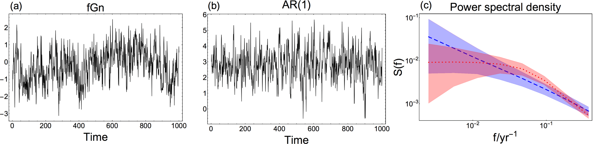
https://www.clim-past.net/14/947/2018/cp-14-947-2018-f01

Figure 1(a) Arbitrary fGn time series with β=0.75. (b) Arbitrary time series of an AR(1) process with parameters estimated from the time series in (a) using maximum likelihood. (c) Log–log spectra showing 95 % confidence ranges based on Monte Carlo ensembles of fGn with β=0.75 (blue shaded area), and AR(1) processes with parameters estimated from the time series in (a) (red, shaded area). Dashed (dotted) lines mark the ensemble means of the fGn (AR(1)) process spectra.

Download

The reconstruction method to be tested, Bayesian Algorithm for Reconstructing Climate Anomalies in Space and Time (BARCAST), is based on a Bayesian hierarchical model (Tingley and Huybers, 2010 a). This is a state-of-the-art paleoclimate reconstruction technique, described in further detail in Sect. 2.1. The motivation for using this particular reconstruction technique in the present study is the contrasting background assumptions for the temporal covariance structure. BARCAST assumes that the temperature evolution follows an AR(1) process in time, while the target data are generated according to the fGn model. The consequences of using an incorrect null hypothesis for the temporal data structure are illustrated in Fig. 1. Here, the original time series in Fig. 1a follows an fGn structure. The corresponding 95 % confidence range of power spectra is plotted in blue in Fig. 1c. Using the incorrect null hypothesis that the data are generated from an AR(1) model, we estimate the AR(1) parameters from the time series in Fig. 1a using maximum likelihood estimation. A realization of an AR(1) process with these parameters is plotted in Fig. 1b, with the 95 % confidence range of power spectra shown in red in Fig. 1c. The characteristic timescale indicating the memory limit of the system is evident as a break in the red AR(1) spectrum. This is an artifact that does not stem from the original data, but simply occurs because an incorrect assumption was used for the temporal covariance structure.

A particular advantage of BARCAST as a probabilistic reconstruction technique lies in its capability to provide an objective error estimate as the result of generating a distribution of solutions for each set of initial conditions. The reconstruction skill of the method has been tested earlier and compared against a few other climate field reconstruction (CFR) techniques using pseudo-proxy experiments. Tingley and Huybers (2010 b) use instrumental temperature data for North America, and construct pseudo-proxy data from some of the longest time series. BARCAST is then compared to the RegEM method used by Mann et al. (2008, 2009). The findings are that BARCAST is more skillful than RegEM if the assumptions for the method are not strongly violated. The uncertainty bands are also narrower. Another pseudo-proxy study is described in Werner et al. (2013), where BARCAST is compared against the canonical correlation analysis (CCA) CFR method. The pseudo-proxies in that paper were constructed from a millennium-long forced run of the NCAR CCSM4 model. The results showed that BARCAST outperformed the CCA method over the entire reconstruction domain, being similar in areas with good data coverage. There is an additional pseudo-proxy study by Gómez-Navarro et al. (2015), targeting precipitation which has a more complex spatial covariance structure than SAT anomalies. In that study, BARCAST was not found to outperform the other methods.

In the following, we describe the methodology of BARCAST and the target data generation in Sect. 2. The spectral estimator used for persistence analyses is also introduced here. Sect. 3 is comprised of an overview of the experiment setup and explains the hypothesis testing procedure. Results are presented in Sect. 4 after performing hypothesis testing in the spectral domain of persistence properties in the local and spatial mean reconstructions. The skill metric results are also summarized. Finally, Sect. 5 discusses the implications of our results and provides concluding remarks.

2 Data and methods

2.1 BARCAST methodology

BARCAST is a climate field reconstruction method, described in detail in Tingley and Huybers (2010 a). It is based on a Bayesian hierarchical model with three levels. The true temperature field in BARCAST, T_t is modeled as an AR(1) process in time. Model equations are defined at the process level:

\begin{matrix} (1) & T_{t} - μ 1 = α (T_{t - 1} - μ 1) + ϵ_{t}, \end{matrix}

where the scalar parameter μ is the mean of the process, α is the AR(1) coefficient and 1 is a vector of ones. The subscript t indexes time in years, and the innovations (increments) ϵ_t are assumed to be independent and identically distributed normal draws $ϵ_{t} \sim N (0, Σ)$ , where

\begin{matrix} (2) & Σ_{i j} = σ^{2} \exp (- ϕ | x_{i} - x_{j} |) \end{matrix}

is the spatial covariance matrix depicting the covariance between locations x_i and x_j.

The spatial e-folding distance is 1∕ϕ and is chosen to be ∼ 1000 km for the target data. This is a conservative estimate resulting in weak spatial correlations for the variability across a continental landmass. (North et al., 2011) estimate that the decorrelation length for a 1-year average of Siberian temperature station data is 3000 km. On the other hand, Tingley and Huybers (2010 a) estimate a decorrelation length of 1800 km for annually mean global land data. They further use annual mean instrumental and proxy data from the North American continent to reconstruct SAT back to 1850, and find a spatial correlation length scale of approximately 3300 km for this BARCAST reconstruction. Werner et al. (2013) use $1 / ϕ \sim$ 1000 km as the mean for the lognormal prior in the BARCAST pseudo-proxy reconstruction for Europe, but the reconstruction has correlation lengths between 6000 and 7000 km. The reconstruction of Werner et al. (2018) has spatial correlation length slightly longer than 1000 km.

On the data level, the observation equations for the instrumental and proxy data are

\begin{matrix} (3) & W_{t} = (\begin{array}{c} H_{I, t} \\ β_{1} \cdot H_{P, t} \end{array}) T_{t} + (\begin{array}{c} e_{I, t} \\ e_{P, t} + β_{0} 1 \end{array}), \end{matrix}

where e_I,t and e_P,t are multivariate normal draws $\sim N (0, τ_{I}^{2} I)$ and $\sim N (0, τ_{P}^{2} I)$ . H_I,t and H_P,t are selection matrices of ones and zeros which at each year select the locations where there are instrumental/proxy data. β₀ and β₁ are parameters representing the bias and scaling factor of the proxy records relative to the temperatures. Note that these two parameters have no relation to the spectral parameter β. The BARCAST parameters are distinguished by their indices, the notation is kept as it is to comply with existing literature.

The remaining level is the prior. Weakly informative but proper prior distributions are specified for the scalar parameters and the temperature field for the first year in the analysis. The priors for all parameters except ϕ are conditionally conjugate, meaning the prior and the posterior distribution has the same parametric form. The Markov Chain Monte Carlo (MCMC) algorithm known as the Gibbs sampler (with one Metropolis step) is used for the posterior simulation (Gelman et al., 2003). Table C1 sums up the prior distributions and the choice of hyperparameters for the scalar parameters in BARCAST. The CFR version applied here has been updated as described in Werner and Tingley (2015). The updated version allows inclusion of proxy records with age uncertainties. This property will not be used here directly, but it implies that proxies of different types may be included. Instead of estimating one single parameter value of $τ_{P}^{2}$ , β₀, β₁, the updated version estimates individual values of the parameters for each proxy record (Werner et al., 2018).

The Metropolis-coupled MCMC algorithm is run for 5000 iterations, running three chains in parallel. Each chain is assumed equally representative for the temperature reconstruction if the parameters converge. There are a number of ways to investigate convergence, for instance one can study the variability in the plots of draws of the model parameters as a function of step number of the sampler, as in Werner et al. (2013). However, a more robust convergence measurement can be achieved when generating more than one chain in parallel. By comparing the within-chain variance to the between-chain variance we get the convergence measurement $\hat{R}$ (Chapter 11 in Gelman et al., 2003). $\hat{R}$ close to 1 indicates convergence for the scalar parameters.

There are numerous reasons why the parameters may fail to converge, including inadequate choice of prior distribution and/or hyperparameters or using an insufficient number of iterations in the MCMC algorithm. It may also be problematic if the spatiotemporal covariance structure of the observations or surrogate data deviate strongly from the model assumption of BARCAST.

BARCAST was used to generate an ensemble of reconstructions, in order to achieve a mean reconstruction as well as uncertainties. In our case, the draws for each temperature field and parameter are thinned so that only every 10 of the 5000 iterations are saved; this secures the independence of the draws.

The output temperature field is reconstructed also in grid cells without observations; this is a unique property compared to other well-known field reconstruction methods such as the regularized expectation maximum technique (RegEM) applied in Mann et al. (2009). Note that the assumptions for BARCAST should generally be different for land and oceanic regions, due to the differences in characteristic timescales and spatiotemporal processes. BARCAST has so far only been configured to handle continental land data (Tingley and Huybers, 2010 a).

2.2 Target data generation

While generating ensembles of synthetic LRM processes in time is straightforward using statistical software packages, it is more complicated to generate a field of persistent processes with prescribed spatial covariance. Below we describe a novel technique that fulfills this goal, which can be extended to include more complicated spatial covariance structures. Such a spatiotemporal field of stochastic processes has many potential applications, both theoretical and practical.

Generation of target data begins with reformulating Eq. (1) so that the temperature evolution is defined from a power law function instead of an AR(1). The continuous-time version of Eq. (1) (with μ=0) is the stochastic (ordinary) differential equation:

\begin{matrix} (4) & d T_{t} = - λ T d t + d W_{t}, \end{matrix}

where $T_{t} = (T_{t, 1}, \dots, T_{t, n})$ and T_t,i is the temperature at time t and spatial position x_i. The noise term $d W_{t} = (d W_{t, 1}, \dots, d W_{t, n})$ is a vector of (dependent) white noise measurements. Spatial dependence is given by Eq. (2) when $ϵ_{t} = W_{t + Δ t} - W_{t}$ and Δt=1 year. If I denotes the identity matrix, the stationary solution of Eq. (4) is

\begin{matrix} (5) & T_{t} = \int_{- \infty}^{t} \exp (- λ I (t - s)) d W_{s}, \end{matrix}

which defines a set of dependent Ornstein–Uhlenbeck processes (the continuous-time versions of AR(1) processes with $α = e^{- λ}$ , $α = 1 - λ$ ). Equation (4) assumes that the system is characterized by a single eigenvalue λ, and consequently that there is only one characteristic timescale 1∕λ. It is well known that surface temperature exhibits variability on a range of characteristic timescales, and more realistic models can be obtained by generalizing the response kernel as a weighted sum of exponential functions (Fredriksen and Rypdal, 2017):

\begin{matrix} (6) & T_{t} = \int_{- \infty}^{t} [\sum_{k} c_{k} \exp (- λ_{k} I (t - s))] d W_{s} . \end{matrix}

An emergent property of the climate system is that the temporal variability is approximately scale invariant (Rypdal and Rypdal, 2014, 2016) and the multi-scale response kernel in Eq. (6) can be approximated by a power law function to yield

\begin{matrix} (7) & T_{t} = \int_{- \infty}^{t} (t - s)^{β / 2 - 1} d W_{s} . \end{matrix}

This expression describes the long memory response to the noise forcing. We note that this should be considered as a formal expression since the stochastic integral is divergent due to the singularity at s=t. Also note that T_t in Eq. (7) in contrast to Eq. (5) is no longer a solution to an ordinary differential equation, but to a fractional differential equation. By neglecting the contribution from the noisy forcing prior to t=0 we obtain

\begin{matrix} (8) & T_{t} = \int_{0}^{t} (t - s)^{β / 2 - 1} d W_{s}, \end{matrix}

which in discrete form can be approximated by

\begin{matrix} (9) & T_{t} = \sum_{s = 0}^{t} (t - s + τ_{0})^{β / 2 - 1} ϵ_{s} . \end{matrix}

The stabilizing term τ₀ is added to avoid the singularity at s=t. The optimal choice would be to choose τ₀ such that the term in the sum arising from s=t represents the integral over the interval $s \in (t - 1, t)$ , i.e.,

τ_{0} = \int_{0}^{τ_{0}} τ^{β / 2 - 1} d τ,

which has the solution $τ_{0} = β / 2$ .

Summations over time steps $s = 1, 2, \dots N$ of (9) results in the matrix product:

T_{t, i} = \sum_{s = 1}^{N} G_{t, s} ϵ_{s, i},

where $G = G_{t, s}$ is the N×N matrix

\begin{matrix} (10) & G_{t, s} = (t - s + β / 2)^{(β / 2 - 1)} Θ (t - s), \end{matrix}

and Θ(t) is the unit step function.

If we for convenience omit the spatial index i from Eq. (10), the model for the target temperature field T at time t can be written in the compressed form

\begin{matrix} (11) & T_{t} = G_{t} ϵ_{t} . \end{matrix}

2.3 Scaling analysis in the spectral domain

The temporal dependencies in the reconstructions are investigated to obtain detailed information about how the reconstruction technique may alter the level of variability on different scales, and how sensitive it is to the proxy data quality. Persistence properties of target data, pseudo-proxies and the reconstructions are compared and analyzed in the spectral domain using the periodogram as the estimator. See Appendix Appendix A for details on how the periodogram is estimated.

Power spectra are visualized in log–log plots since the spectral exponent then can be estimated by a simple linear fit to the spectrum. The raw and log-binned periodograms are plotted, and β is estimated from the latter. Log binning of the periodogram is used here for analytical purposes, since it is useful with a representation where all frequencies are weighted equally with respect to their contributions to the total variance.

It is also possible to use other estimators for scaling analysis, such as the detrended fluctuation analysis (DFA; Peng et al., 1994), or wavelet variance analysis (Malamud and Turcotte, 1999). One can argue for the superiority of methods other than PSD or the use of a multi-method approach. However, we consider the spectral analysis to be adequate for our purpose and refer the reader to Rypdal et al. (2013) and Nilsen et al. (2016) for discussions on selected estimators for scaling analysis.

3 Experiment setup

The experiment domain configuration is selected to resemble that of the continental landmass of Europe, with N=56 grid cells of size $5^{\circ} \times 5^{\circ}$ . The reconstruction period is 1000 years. reflecting the last millennium. The reconstruction region and period are inspired by the BARCAST reconstructions in Werner et al. (2013); Luterbacher et al. (2016) and approximate the density of instrumental and proxy data in reconstructions of the European climate of the last millennium. The temporal resolution for all types of data is annual. By design, the target fGn data are meant to be an analogue of the unforced SAT field. We will study both the field and spatial mean reconstruction.

Pseudo-instrumental data cover the entire reconstruction region for the time period 850–1000 and are identical to the noise-free values of the true target variables. The spatial distribution of the pseudo-proxy network is highly idealized as illustrated in Fig. 2, the data covers every fourth grid cell for the time period 1–1000. The pseudo-proxies are constructed by perturbing the target data with white noise according to Eq. (3). The variance of the proxy observations is $τ_{P}^{2}$ , and the SNR is calculated as

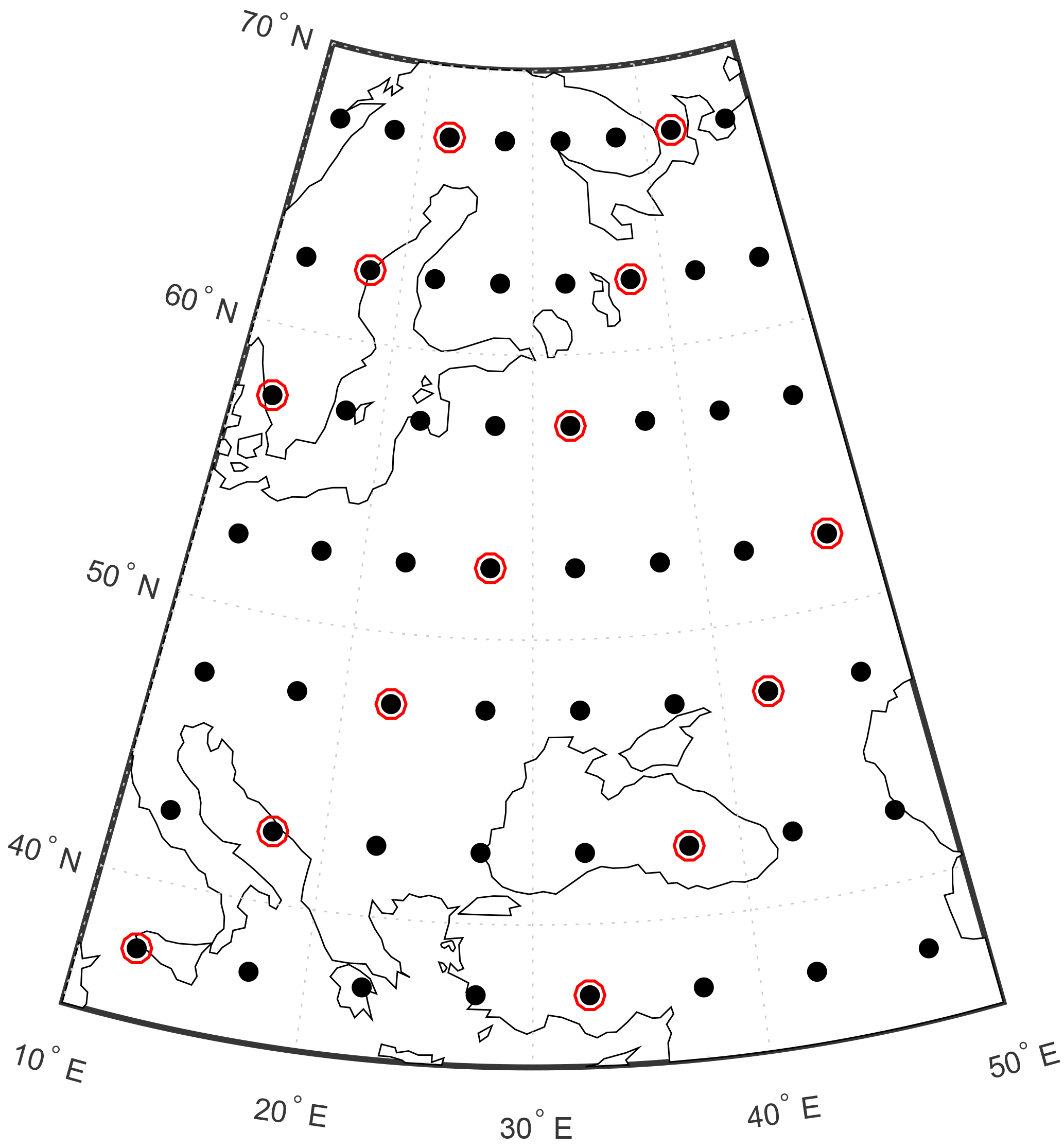
\begin{matrix} (12) & SNR = \frac{β_{1}^{2} Var (T_{t})}{τ_{P}^{2}} . \end{matrix}

https://www.clim-past.net/14/947/2018/cp-14-947-2018-f02

Figure 2The spatial domain of the reconstruction experiments. Dots mark locations of instrumental sites, proxy sites are highlighted by red circles. The superimposed map of Europe provides a spatial scale.

Download

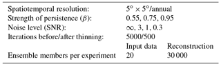
Our set of experiments is summarized in Table 1 and comprises target data with three different strengths of persistence, $β = 0.55, 0.75, 0.95$ and pseudo-proxies with SNR $= \infty, 3, 1$ , and 0.3. In total, 20 realizations of target pseudo-proxy and pseudo-instrumental data are generated for each combination of β and SNR and used as input to BARCAST. The reconstruction method is probabilistic and generates ensembles of reconstructions for each input data realization. In total, 30 000 ensemble members are constructed for every parameter setup.

Table 1Summary of the experiment setup.

Download Print Version | Download XLSX

3.1 Hypothesis testing

Hypothesis testing in the spectral domain is used to determine which pseudo-proxy/reconstructed data sets can be classified as fGn with the prescribed scaling parameter, or as AR(1) with parameter α estimated from BARCAST. The power spectrum for each ensemble member of the local/spatial mean reconstructions is estimated, and the mean power spectrum is then used for further analyses. The first null hypothesis is that the data sets under study can be described using an fGn with the prescribed scaling parameter for the target data at all frequencies, $β_{target} = 0.55, 0.75$ , 0.95, respectively. For testing we generate a Monte Carlo ensemble of fGn series with a value of the scaling parameter identical to the target data. The power spectrum of each ensemble member is estimated, and the confidence range for the theoretical spectrum is then calculated using the 2.5 and 97.5 quantiles of the log-binned periodograms of the Monte Carlo ensemble. The null hypothesis is rejected if the log-binned mean spectrum of the data is outside of the confidence range for the fGn model at any point.

The second null hypothesis tested is that the data can be described as an AR(1) process at all frequencies, with the parameter α estimated from BARCAST. Distributions for all scalar parameters including the AR(1) parameter α are provided through the reconstruction algorithm. The mean of this parameter was used to generate a Monte Carlo ensemble of AR(1) processes. The Monte Carlo ensemble and the confidence range are then based on log-binned periodograms for this theoretical AR(1) process.

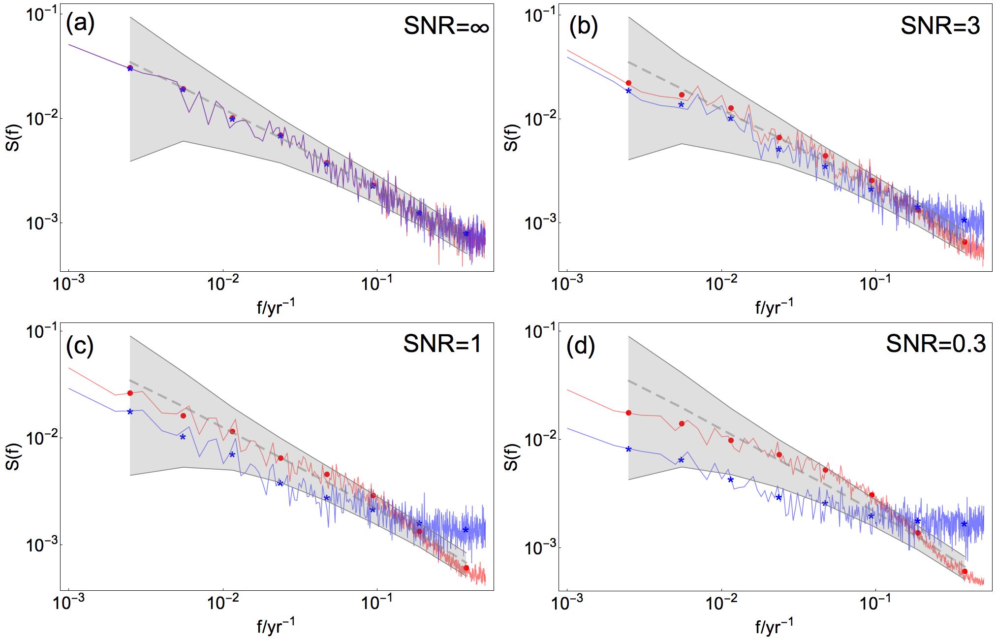
https://www.clim-past.net/14/947/2018/cp-14-947-2018-f03

Figure 3Mean raw and log-binned PSD for pseudo-proxy data (blue curve and asterisks, respectively) and reconstruction at the same site (red curve and dots, respectively) generated from β_target= 0.75 and different SNR indicated in (a)–(d). Colored gray shading and dashed, gray lines indicate 95 % confidence range and the ensemble mean, respectively, for a Monte Carlo ensemble of fGn with β= 0.75.

Download

Figure 3 presents an example of the hypothesis testing procedure. The fGn 95 % confidence range is plotted as a shaded gray area in the log–log plot together with the mean raw and mean log-binned periodograms for the data to be tested. Blue curve and dots represent mean raw and log-binned PSD for pseudo-proxy data, and red curve and dots represent mean raw and log-binned PSD for reconstructed data. The gray, dotted line is the ensemble mean.

The two null hypotheses provide no restrictions on the normalization of the fGn and AR(1) data used to generate the Monte Carlo ensembles. In particular, they do not have to be standardized in the same manner as the pseudo-proxy/reconstructed data. This makes the experiments more flexible, as the confidence range of the Monte Carlo ensemble can be shifted vertically to better accommodate the data under study. A standard normalization of data includes subtracting the mean and normalizing by the standard deviation. This was sufficient to support the null hypotheses in many of our experiments. A different normalization had to be used in other experiments.

4 Results

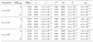
BARCAST successfully estimates posterior distributions for all reconstructed temperature fields and scalar parameters. Convergence is reached for the scalar parameters despite the inconsistency of the input data temporal covariance structure with the default assumption of BARCAST. Table C2 lists the true parameter values used for the target data generation, and Table C3 summarizes the mean of the posterior distributions estimated from BARCAST. Studying the parameter dependencies, it is clear that the posterior distributions of α and σ² depend on the prescribed β and, to a lesser extent, SNR for the target data. Instead of listing the posterior distributions of $τ_{P}^{2}$ and β₁ we have estimated the local reconstructed SNR at each proxy location using Eq. (12).

Further results concern the spectral analyses and skill metrics. All references to spectra in the following correspond to mean spectra. Analyses of the reconstruction skill presented below are performed on a grid point basis, and for the correlation and RMSE also for the spatial mean reconstruction. While the latter provides an aggregate summary of the method's ability to reproduce specified properties of the climate process on a global scale, the former evaluates BARCAST's spatial performance.

4.1 Isolated effects of added proxy noise on scaling properties in the input data

The scaling properties of the input data have already been modified when the target data are perturbed with white noise to generate pseudo-proxies. The power spectra shown in blue in Fig. 3 are used to illustrate these effects for one arbitrary proxy location and β=0.75. Figure 3a shows the pseudo-proxy spectrum for SNR =∞, which is the unperturbed fGn signal corresponding to ideal proxies. Figure 3b–d show pseudo-proxy spectra for SNR = 3, 1, 0.3, respectively. The effect of added white noise in the spectral domain is manifested as flattening of the high-frequency part of the spectrum equal to β=0, and a gradual transition to higher β for lower frequencies. The results for β_target=0.55 and 0.95 are similar (figures not shown).

4.2 Memory properties in the field reconstruction

Hypothesis testing was performed in the spectral domain for the field reconstructions, with the two null hypotheses formulated as follows:

The reconstruction is consistent with the fGn structure in the target data for all frequencies.
The reconstruction is consistent with the AR(1) model used in BARCAST for all frequencies.

Table 2 summarizes the results for all experiment configurations at local grid cells, both directly at and between proxy locations. Figure 3 shows the mean power spectra generated for one arbitrary proxy grid cell of the reconstruction in red. The fGn model is adequate for SNR = ∞, 3 and 1, shown in Fig. 3a–c. For the lowest SNR presented in panel (d), the reconstruction spectrum falls outside the confidence range of the theoretical spectrum for one single log-binned point. Not unexpectedly, the difference in shape of the PSD between the pseudo-proxy and reconstructed spectra increases with decreasing SNR. The difference is largest for the noisiest proxies with SNR = 0.3. This figure does not show the hypothesis testing for the reconstructed spectrum using the AR(1) process null hypothesis. Results show that this null hypothesis is rejected for all cases except SNR = 0.3.

Table 2Hypothesis testing results for local reconstructed data compared to Monte Carlo ensembles of fGn and AR(1) processes. The “x” mark in the table indicates that the null hypothesis cannot be rejected. Null hypotheses are 1: the reconstruction is consistent with the fGn structure in the target data for all frequencies; 2: the reconstruction is consistent with the AR(1) assumption from BARCAST for all frequencies.

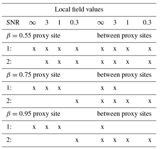
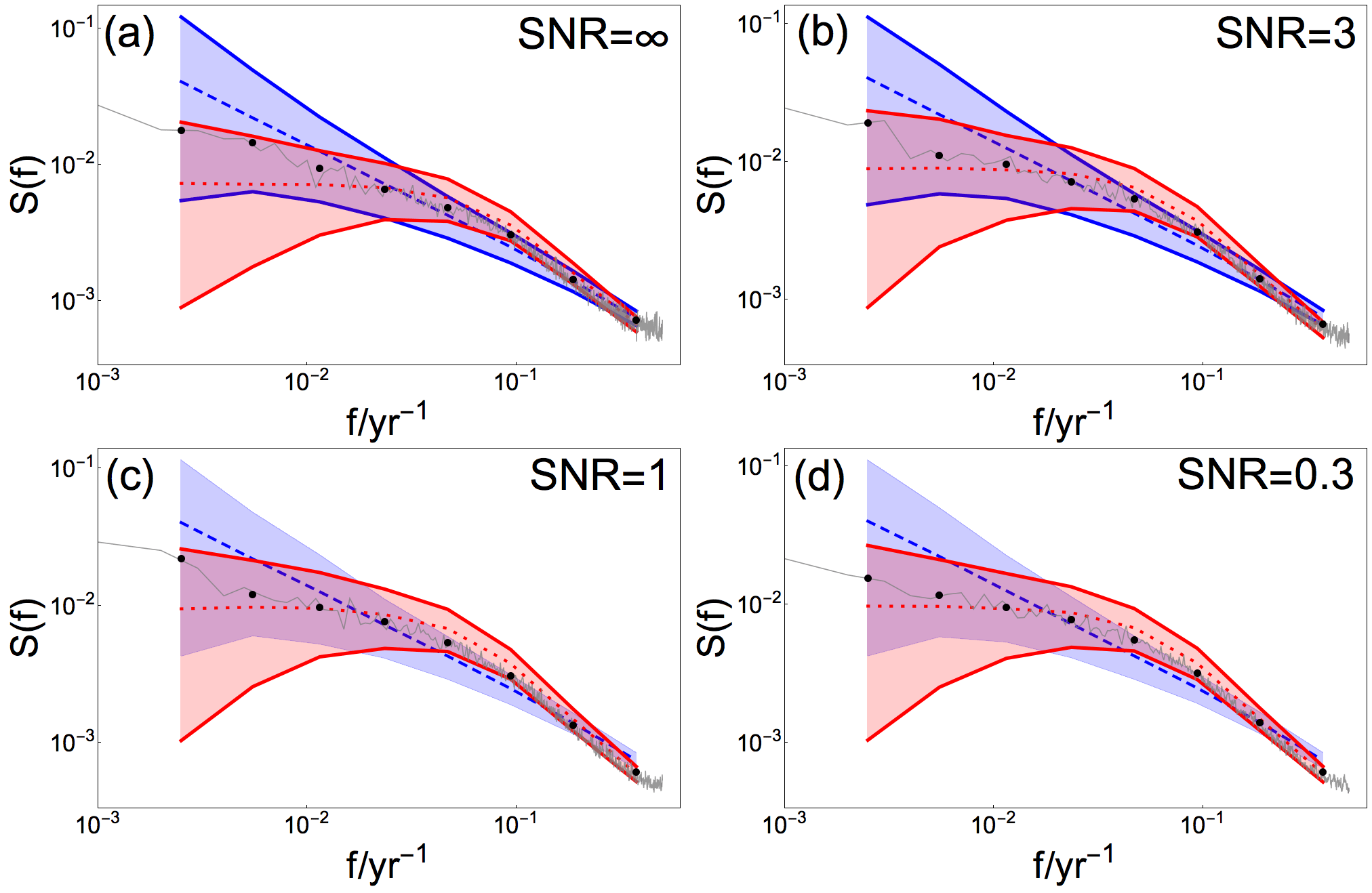
Download Print Version | Download XLSX

https://www.clim-past.net/14/947/2018/cp-14-947-2018-f04

Figure 4Mean raw and log-binned PSD for local reconstructed data at a site between proxies (gray curve and dots, respectively) generated from β_target= 0.75 and different SNR indicated in (a)–(d). Colored shading and dashed/dotted lines indicate 95 % confidence range and the ensemble mean, respectively, for a Monte Carlo ensemble of fGn with β= 0.75 (blue) and of AR(1) processes with α estimated from BARCAST (red). The confidence ranges found consistent with the data are drawn with solid lines.

Download

The hypothesis testing results vary moderately between the individual grid cells. PSD analyses of the local reconstructions using the same β but in an arbitrary non-proxy location are displayed in Fig. 4. Here, the reconstructed mean spectrum is plotted in gray together with both the fGn 95 % confidence range (blue) and the AR(1) confidence range (red). Hypothesis testing using null hypothesis 1 and 2 is performed systematically. Wherever the reconstructed log-binned spectrum is consistent with the fGn/AR(1) model, the edges of the associated confidence range are plotted with solid lines. We find that all reconstructed log-binned spectra are consistent with the AR(1) model, and for SNR = ∞ and 3 the reconstructions are also consistent with the fGn model.

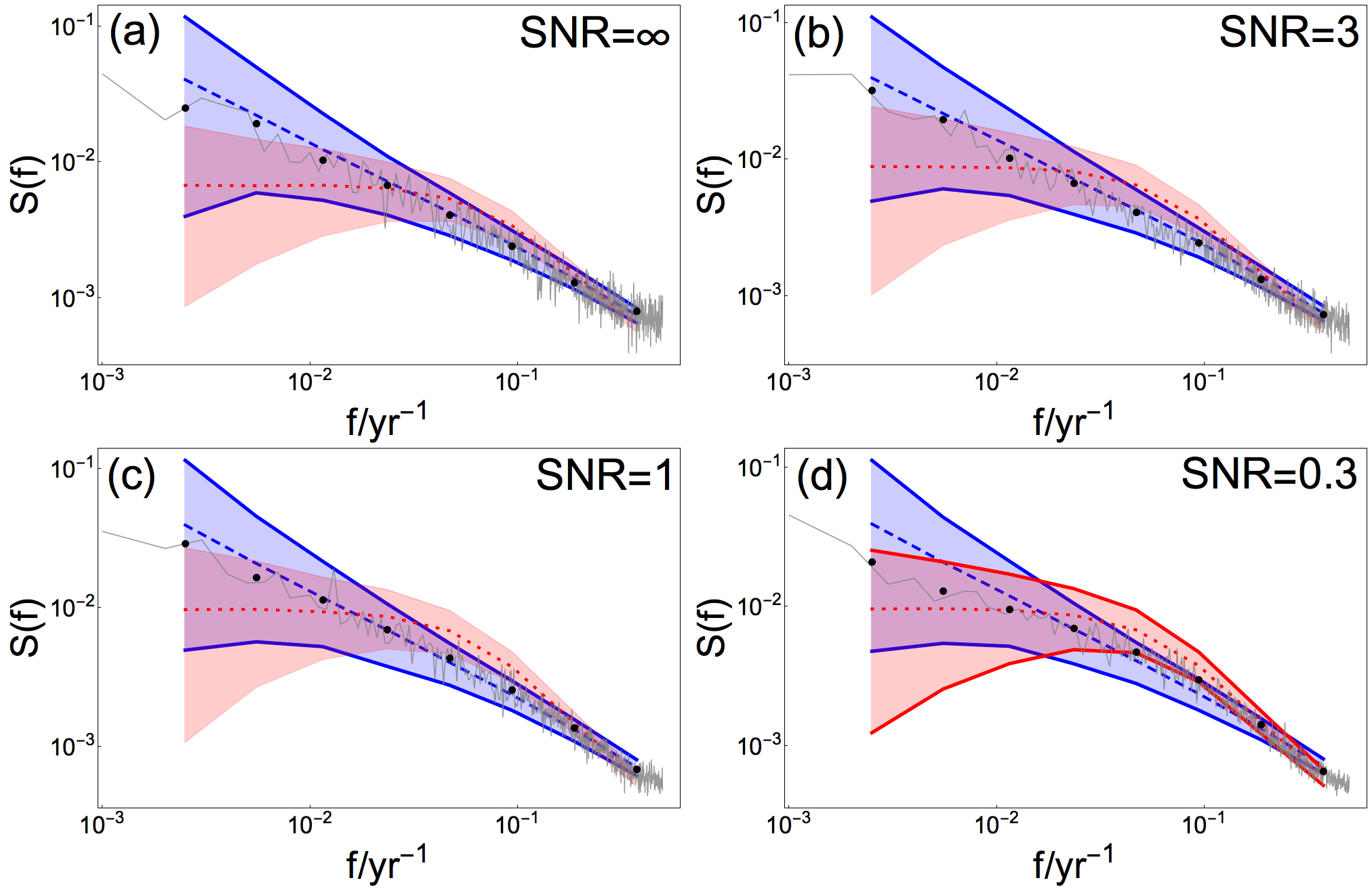
https://www.clim-past.net/14/947/2018/cp-14-947-2018-f05

Figure 5Mean raw and log-binned PSD for the spatial mean reconstruction (gray curve and dots, respectively), generated from β_target= 0.75 and different SNR indicated in (a)–(d). Colored shading and dashed/dotted lines indicate 95 % confidence range and the ensemble mean, respectively, for a Monte Carlo ensemble of fGn with β= 0.75 (blue) and of AR(1) processes with α estimated from BARCAST (red). The confidence ranges found consistent with the data are drawn with solid lines.

Download

4.3 Memory properties in the spatial mean reconstruction

The spatial mean reconstruction is calculated as the mean of the local reconstructions for all grid cells considered, weighted by the areas of the grid cells. The reconstruction region considered is 37.5–67.5^∘ N, 12.5–47.5^∘ E, as shown in Fig. 2. Figure 5 shows the raw and log-binned periodogram of the spatial mean reconstruction for β_target=0.75 in gray, together with the 95 % confidence range of fGn generated with β=0.75 (blue) and AR(1) confidence range (red). All hypothesis testing results for the spatial mean reconstruction are summarized in Table 3. Results show that the fGn null hypothesis is suitable for all values of β and SNR, while the AR(1) process null hypothesis is also supported for the case $β = 0.55, 0.75$ , SNR = 0.3.

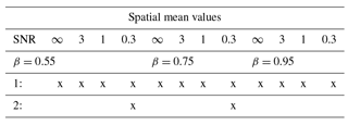
Table 3Hypothesis testing results for spatial mean reconstructed data compared to Monte Carlo ensembles of fGn and AR(1) processes. The null hypotheses 1 and 2 are the same as in Table 2, and the “x” has the same meaning.

Download Print Version | Download XLSX

4.4 Effects from BARCAST on the reconstructed signal variance

The power spectra can also be used to gain information about the fraction of variance lost/gained in the reconstruction compared with the target. This fraction is in some sense the bias of the variance, and was found by integrating the spectra of the input and output data over frequency. The spatial mean target/reconstructions were used, and the mean log-binned spectra. The total power in the spatial mean reconstruction and the target were estimated, and the ratio of the two provides the under/overestimation of the variance: $R_{Var} = \frac{Var (T_{t (rec)})}{Var (T_{t (target)})}$ . A ratio less than unity implies that the reconstructed variance is underestimated compared with the target. Our analyses for the total variance reveal that the ratio varies between 0.83 and 1.05 for the different experiments and typically decreases for increasing noise levels. How much the ratio decreases with SNR depends on β, with higher ratios for higher β values. For example, R∼1 for all β, SNR =∞ and progressively decreases to R=0.83, 0.89, 0.94 for SNR = 0.3, $β = 0.55, 0.75, 0.95$ , respectively. In other terms, there are larger variance losses in the reconstruction for smaller values of β than for higher β. We also divided the spectra into three different frequency ranges as shown in Fig. 6 to test if the fraction of variance lost/gained is frequency dependent. The sections separate low frequencies corresponding approximately to centennial timescales, middle frequencies corresponding to timescales between decades and centuries and high frequencies corresponding to timescales shorter than decadal. The results show no systematic differences between the frequency ranges associated with the parameter configuration.

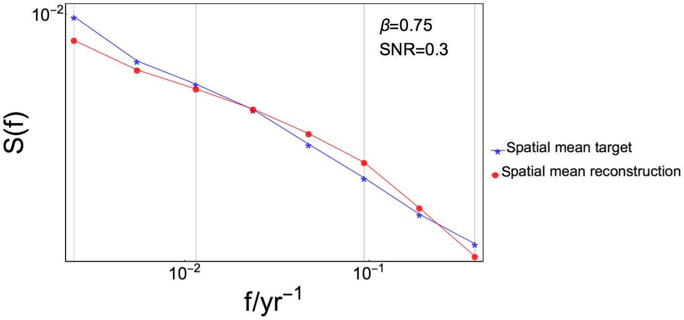
https://www.clim-past.net/14/947/2018/cp-14-947-2018-f06

Figure 6Log–log plot showing log-binned power spectra of spatial mean target (blue) and reconstruction (red) for one experiment. Vertical gray lines mark the frequency ranges used to estimate bias of variance as referred to in Sect. 4.4.

Download

https://www.clim-past.net/14/947/2018/cp-14-947-2018-f07

Figure 7Local correlation coefficient between reconstructed temperature field and target field for the verification period (ensemble mean). The box plots left of the color bars indicate the distribution of grid point correlation coefficients. β= 0.75

Download

https://www.clim-past.net/14/947/2018/cp-14-947-2018-f08

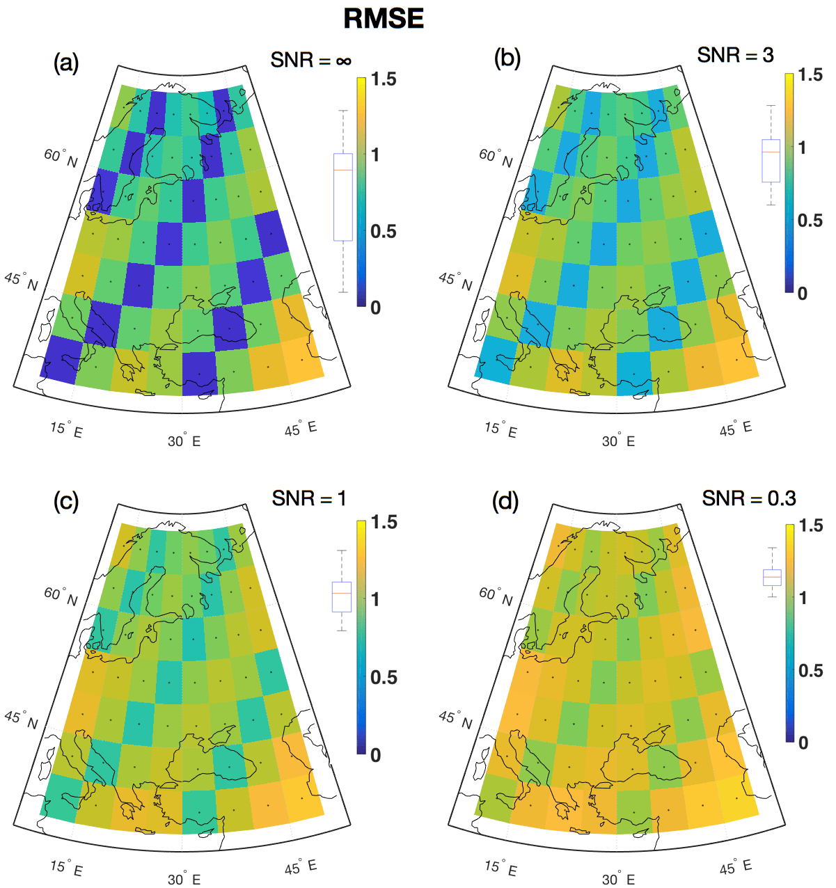
Figure 8Local RMSE between reconstructed temperature field and target field for the verification period. The box plots left of the color bars indicate the distribution of grid point correlation coefficients. β= 0.75.

Download

https://www.clim-past.net/14/947/2018/cp-14-947-2018-f09

Figure 9Local ${\overline{CRPS}}_{pot}$ between reconstructed temperature field and target field for the verification period. The box plots left of the color bars indicate the distribution of grid point correlation coefficients. β= 0.75.

Download

4.5 Assessment of reconstruction skill

It is common practice in paleoclimatology to evaluate reconstruction skill using metrics such as the Pearson's correlation coefficient r, the RMSE, the coefficient of efficiency (CE) and reduction of error (RE; Smerdon et al., 2011; Wang et al., 2014). The two former skill metrics will be used in this study, but the CE and RE metrics are not proper scoring rules and are therefore unsuitable for ensemble-based reconstructions in general (Gneiting and Raftery, 2007; Tipton et al., 2015); see also Appendix Appendix B. Instead, the continuous ranked probability score (CRPS) will be used (Gneiting and Raftery, 2007). The metric was used specifically for probabilistic climate reconstructions in Tipton et al. (2015); Werner and Tingley (2015); Werner et al. (2018). Since the CRPS, its average and subcomponents are less well known than the two former skill metrics, we define these terms in Appendix Appendix B and refer the reader to Gneiting and Raftery (2007) and Hersbach (2000) for further details. CRPS results below are shown for the $\overline{CRPS}$ represented via the sum of the subcomponents ${\overline{CRPS}}_{pot}$ and $\overline{Reli}$ score.

4.5.1 Skill measurement results

Figures 7–9 display the spatial distribution of the ensemble mean skill metrics for the experiment β=0.75 and all noise levels. All figures show a spatial pattern of dependence on the proxy availability, with the best skill attained at proxy sites. This is the most important result for all the spatially distributed skill metrics. For the BARCAST CFR method, the signal at locations distant from proxy information by design cannot be skillfully reconstructed, as the amount of shared information on the target climate field between the two locations decreases exponentially with distance (Werner et al., 2013). See Sect. 5 for further details on the relation between skill and co-localization of proxy data.

Figure 7 shows the local correlation coefficient r between the target and the localized reconstruction for the verification period 2–1849. The correlation is highest for the ideal proxy experiment in Fig. 7a, and gradually decreases at all locations as the noise level rises in panels (b)–(d). Figure 8 shows the local RMSE. Note that Figs. 8–9 use the same color bar as in Fig. 7, but best skill is achieved where the RMSE/ ${\overline{CRPS}}_{pot}$ is low. Figure 9 shows the distribution of ${\overline{CRPS}}_{pot}$ . The contribution from $\overline{Reli}$ is generally $< 1 \times 10^{- 2}$ , indicating excellent correspondence between the predicted and the reconstructed confidence intervals. The ${\overline{CRPS}}_{pot}$ therefore dominates the average CRPS metric. The minimum estimate for the ${\overline{CRPS}}_{pot}$ at proxy locations in Fig. 9a is $2 \times 10^{- 2}$ , indicating a low error between the temporally averaged reconstruction and the target. For the remaining locations in Fig. 9a–d, the estimates are between 0.24 and 0.55 given in the same unit as the target variable. The temperature unit has not been given for our reconstructions, but for real-world reconstructions the unit will typically be degrees Celsius (^∘C) or Kelvin (K).

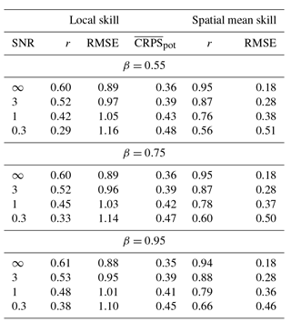
Table 4 summarizes the median local skill for all experiments. BARCAST is in general able to reconstruct major features of the target field. A general conclusion that can be drawn is that the skill metrics vary with SNR, but are less sensitive to the value of β. For the highest noise level SNR = 0.3, the values obtained for r and the RMSE are in line with those listed in Table 1 of Werner et al. (2013).

Table 4 also sums up the ensemble median skill values of r and RMSE for the spatial mean reconstructions. The skill is considerably better than for the local field reconstructions.

5 Discussion

In this study we have tested the capability of BARCAST to preserve temporal LRM properties of reconstructed data. Pseudo-proxy and pseudo-instrumental data were generated with a prescribed spatial covariance structure and LRM temporal persistence using a new method. The data were then used as input to the BARCAST reconstruction algorithm, which by design use an AR(1) model for temporal dependencies in the input/output data. The spatiotemporal availability of observational data was kept the same for all experiments in order to isolate the effect of the added noise level and the strength of persistence in the target data. The mean spectra of the reconstructions were tested against the null hypotheses that the reconstructed data can be represented as LRM processes using the parameters specified for the target data, or as AR(1) processes using the parameter estimated from BARCAST.

We found that despite the default assumptions in BARCAST, not all local and spatial mean reconstructions were consistent with the AR(1) model. Figures 3–5 and Tables 2–3 summarize the hypothesis testing results; the local reconstructions at grid cells between proxy locations follow to large extent the AR(1) model, while the local reconstructions directly at proxy locations are more similar to the original fGn data. However, the simulated proxy quality is crucial for the spectral shape of the local reconstructions, with higher noise levels indicating better agreement with the AR(1) model than fGn.

All spatial mean reconstructions are consistent with the fGn process null hypothesis according to Table 3. For the two cases $β = 0.55, 0.75$ , SNR = 0.3, the spatial mean reconstructions are also consistent with the AR(1) process null hypothesis. This is clear from the spatial mean reconstruction spectra (gray curves in Fig. 5) and from comparing the hypothesis testing results in Tables 2 and 3. The improvement in scaling behavior with spatial averaging is expected, as the small-scale variability denoted by ϵ_t in Eq. (11) is averaged out. Eliminating local disturbances naturally results in a more coherent signal. However, the spatial mean of the target data set does not have a significantly higher β than local target values. This is due to the relatively short spatial correlation length chosen: $1 / ϕ = 1000$ km. In observed temperature data, spatial averaging tends to increase the scaling parameter β (Fredriksen and Rypdal, 2016).

The power spectra in Figs. 3–5b–d show that the temporal covariance structure of the reconstructions is altered compared with the target data for all experiments where noisy input data were used. Furthermore, the spectra of the pseudo-proxies in Fig. 3b–d all deviate from the target in the high-frequency range, but for a different reason. The pseudo-proxy data deviate from the target due to the white proxy noise component, while the reconstruction deviate because BARCAST quantifies the proxy noise from an AR(1) assumption. Real-world proxy data are generally noisy, and the noise level is normally at the high end of the range studied here. We demonstrate that the variability level of the reconstructions does not exclusively reflect the characteristics of the target data, but is also influenced by the fitting of noisy data to a model that is not necessarily correct. At present, there exists no reconstruction technique assuming explicitly that the climate variable follows an LRM process.

In addition to BARCAST, other reconstruction techniques that may experience similar deficiencies for LRM target data are the regularized expectation–maximization algorithm (RegEM; Schneider, 2001; Mann et al., 2007) and all related models (CCA, PCA, GraphEM). These models assume observations at subsequent years are independent (Tingley and Huybers, 2010 b). The assumption of temporal independence corresponds to yet another incorrect statistical model for our target data, a white noise process in time. Note that for target variables/data sets consistent with a white noise process, these types of reconstruction methods are appropriate, as demonstrated using the truncated empirical orthogonal function (EOF) principal component spatial regression methodology on precipitation data in Wahl et al. (2017).

When an incorrect statistical model is used to reconstruct a climate signal, the temporal correlation structure is likely to be deteriorated in the process. For the range of different reconstructions available, such effects may contribute to discussions on a number of questions under study, including the possible existence of different scaling regimes in paleoclimate; see Huybers and Curry (2006); Lovejoy and Schertzer (2012); Rypdal and Rypdal (2016); Nilsen et al. (2016).

The criteria for the hypothesis testing used in this study are strict, and may be modified if reasonable arguments are provided. For example, if the first null hypothesis used here was modified so that only the low-frequency components of the spectra were required to fall within the confidence ranges, more of the reconstructions would be consistent with the fGn model. However, from studying the spectra in Figs. 3–5, it is generally unclear where one should set a threshold, since the spectra show a gradual change with a lack of any abrupt breaks. Considering real-world proxy records, the noise color and level is generally unknown or not quantified. We know there are certain sources of noise influencing different frequency ranges that are unrelated to climate, but it is difficult to decide when the noise becomes negligible compared with the effects of climate driven processes. The decision to use all frequencies for the hypothesis testing in this idealized study is therefore a conservative and objective choice.

The skill metrics used to validate the reconstruction skill are the Pearson's correlation coefficient r, the RMSE and $\overline{CRPS}$ , the latter divided into the ${\overline{CRPS}}_{pot}$ and the $\overline{Reli}$ . Skill metric results are illustrated in Figs. 7–9 and summarized in Table 4. The reconstruction skill is sensitive to the proxy quality, and highest at sites with co-localized proxy information. This is an expected result, due to the BARCAST model formulation and our choice of a relatively short decorrelation length $1 / ϕ \sim 1000$ km. Contrasting results of high skill away from proxy sites and poor skill close to proxy sites have been documented in Wahl et al. (2017), although care must be taken in the comparison as that paper used a different reconstruction methodology (truncated EOF principal component spatial regression) and the target variable was precipitation/hydroclimate instead of SAT. Without performing dedicated pseudo-proxy experiments it is difficult to resolve the main cause of these contrasting results for spatial skill.

5.1 Implications for real proxy data

The spectral shape of the input pseudo-proxy data plotted in blue in Fig. 3 is similar to the spectral shape of observed proxy data as observed in, for example, some types of tree-ring records (Franke et al., 2013; Zhang et al., 2015; Werner et al., 2018). In particular, Franke et al. (2013) and Zhang et al. (2015) found that the scaling parameters β were higher for tree-ring-based reconstructions than for the corresponding instrumental data for the same region. Werner et al. (2018) present a new spatial SAT reconstruction for the Arctic, using the BARCAST methodology. The analyses shown in Fig. A4 demonstrate that several of the tree-ring records could not be categorized as either AR(1) or scaling processes, but featured spectra similar to the pseudo-proxy spectrum in our Fig. 3c–d. We hypothesize that the possible mechanism(s) altering the variability can be due to effects of the tree-ring processing techniques, specifically the methods applied to eliminate the biological tree aging effect on the growth of the trees (Cook et al., 1995). The actual tree-ring width is a superposition of the age-dependent curve, which is individual for a tree, and a signal that can often be associated with climatic effects on the tree growth process. To correct for the biological age-effect, the raw tree-ring growth values are often transformed into proxy indices using the regional curve standardization technique (RCS; Briffa et al., 1992; Cook et al., 1995), age band decomposition (ABD; Briffa et al., 2001), the signal-free processing (Melvin and Briffa, 2008) or other techniques. These techniques attempt to eliminate biological age effects on tree-ring growth while preserving low-frequency variability. As an example, consider the RCS processing of tree-ring width as a function of age (Helama et al., 2017). For a number of individual tree-ring records, each record is aligned according to its biological years. The mean of all the series is then modeled as a negative exponential function (the RCS curve). To construct the RCS chronology, the raw, individual tree-ring width curves are divided by the mean RCS curve for the full region. The RCS chronology is then the average of the index individual records. It is likely that the shape of a particular tree-ring width spectrum reflects the uncertainty in the standardization curve, which is expected to be largest at the timescales corresponding to the initial stage of a tree growth, where the slope of the growth curve is generally steeper (i.e., of the order of a few decades). In particular, there may be slightly different climate processes affecting the growth of different trees, causing localized nonlinearities that limit the representativeness of the derived chronology. We therefore suggest that the observed excess of LRM properties in some of the tree-ring-based proxy records could be an artifact of the fitting procedure.

Table 4Median local skill measurements

Download Print Version | Download XLSX

Our study further suggests that for a proxy network of high quality and density, exhibiting LRM properties, the BARCAST methodology is capable, without modification, of constructing skillful reconstructions with LRM preserved across the region. This is because the data information overwhelms the vague priors. The availability of well-documented proxy records therefore helps the analyst select an appropriate reconstruction method based on the input data. For quantification and assessment of real-world proxy quality, forward proxy modeling is a powerful tool that models proxy growth/deposition instead of the target variable evolution, also taking known proxy uncertainties and biases into consideration. See for example Dee et al. (2017) for a comprehensive study on terrestrial proxy system modeling, and Dolman and Laepple (2018) for a study on forward modeling of sediment-based proxies.

6 Concluding remarks

Several extensions to the presented work appear relevant for future studies, including (a) implementing external forcing and responses to this forcing in the target data to make the numerical experiments more realistic, (b) generating target data using a more complex model than described in Sect. 2.2 and (c) reformulating BARCAST model Eqs. (1)–(2) to account for LRM properties in the target data. In addition, there is the possibility of repeating the experiments from this study using a different reconstruction technique, and experiments with more complicated spatiotemporal design of the multi-proxy network can also be considered (Smerdon, 2012; Wang et al., 2014).

The alternatives (a) and (b) can be implemented together. Relevant advancements for target data generation can be obtained using the class of stochastic–diffusive models, such as the models described in North et al. (2011); Rypdal et al. (2015). The alternative method for generating spatial covariance stands in contrast to what is done in the present study. The data generation technique used in this paper and also in Werner et al. (2014) and Werner and Tingley (2015) generates a signal without spatial dynamics, where the spatial covariance is defined through the noise term. On the other hand, the stochastic–diffusive models generate the spatial covariance through the diffusion, without spatial structure in the noise term. The latter model type may be considered more physically correct and intuitive than the simplistic model used here. North et al. (2011) use an exponential model for the temporal covariance structure, while Rypdal et al. (2015) use an LRM model.

For the BARCAST CFR methodology, reformulation of model Eqs. (1)–(2) would drastically improve the performance in our experiments. However, at present we cannot guarantee that modifications favoring LRM are practically feasible in the context of a Bayesian hierarchical model, due to higher computational demands. Changing the AR(1) model assumption to instead account for LRM would in the best scenario slow the algorithm down substantially, and in the worst scenario it would not converge at all. Some cut-off timescale would have to be chosen to ensure convergence. Regarding the spatial covariance structure, accounting for teleconnections introduces similar computational challenges. The more general Matérn covariance family form (Tingley and Huybers, 2010 a) has already been implemented for BARCAST, but was not used in this study. Another problem is the potential temporal instability of teleconnections; it is possible that major climate modes might have changed their configuration through time. Therefore, setting additional a priori constraints on the model may not be considered justified. The use of exponential covariance structure appears to be a conservative choice in such a situation.

The pseudo-proxy study presented here sets a powerful example for how to construct and utilize an experimental structure to isolate specific properties of paleoclimate reconstruction techniques. The generation of the input data requires far less computation power and time than for GCM paleoclimatic simulations, but also results in less realistic target temperature fields. We demonstrate that there are many areas of use for these types of data, including statistical modeling and hypothesis testing.

Data availability

Data and codes are available on request, including BARCAST code package.

Appendix A: Estimation of the periodogram

The periodogram is defined here in terms of the discrete Fourier transform H_m as (Malamud and Turcotte, 1999)

S (f_{m}) = (\frac{2}{N}) | H_{m} |^{2}, m = 1, 2, \dots, N / 2,

for evenly sampled time series $x_{1}, x_{2}, \dots . x_{N}$ . The sampling time is an arbitrary time unit, and the frequency is measured in cycles per time unit: $f_{m} = \frac{m}{N} \cdot Δ f = \frac{1}{N}$ is the frequency resolution and the smallest frequency which can be represented in the spectrum.

Appendix B: Continuous ranked probability score (CRPS) for a reconstruction ensemble

For probabilistic forecasts, scoring rules are used to measure the forecast accuracy, and proper scoring rules secure that the maximum reward is given when the true probability distribution is reported. In contrast, the reduction of error (RE) and coefficient of efficiency (CE) are improper scoring rules, meaning they measure the accuracy of a forecast, but the maximum score is not necessarily given if the true probability distribution is reported. For climate reconstructions, RE = 1 and CE = 1 imply a deterministic forecast, the maximum score is obtained when the mean (a point measurement) within the probability distribution P is used instead of the predictive distribution P itself.

The concept behind the CRPS is to provide a metric of the distance between the predicted (forecasted) and occurred (observed) cumulative distribution functions of the variable of interest. The lowest possible value for the metric corresponding to a perfect forecast is therefore CRPS = 0. Following Sect. 4b of Hersbach (2000) (elaborated for clarity), the definition of the CRPS and its subcomponents can be defined as follows:

\begin{matrix} (B1) & CRPS (P, x_{target}) = \int_{- \infty}^{\infty} [P (x) - Θ (x - x_{target})]^{2} d x, \end{matrix}

where x is the variable of interest, x_target denotes target (validation) data, Θ is the unit step function and P(x) is the cumulative distribution function of the forecast ensemble with a probability density function (PDF) of ρ(y):

\begin{matrix} (B2) & P (x) = \int_{- \infty}^{x} ρ (y) d y . \end{matrix}

In the case of a reconstruction ensemble at each spatial location j and time step t (omitted for convenience), the CRPS can be evaluated as

\begin{matrix} (B3) & CPRS = \sum_{i = 0}^{N} \int_{x_{i}}^{x_{i + 1}} [\frac{i}{N} - Θ (x - x_{target})]^{2} d x, \end{matrix}

where $x_{i} < x < x_{i + 1}$ refers to members of the locally ordered reconstruction ensemble of length N. For this study, x corresponds to the ensemble of local reconstructed values of T.

For the average over K time and/or grid points, the average CRPS ( $\overline{CPRS}$ ) is defined as a weighted sum with equal weights, yielding

\begin{matrix} (B4) & \overline{CPRS} = \sum_{i = 0}^{N} {\overline{g}}_{i} [(1 - {\overline{o}}_{i}) {(\frac{i}{N})}^{2} + {\overline{o}}_{i} {(1 - \frac{i}{N})}^{2}] . \end{matrix}

Here, ${\overline{g}}_{i}$ and ${\overline{o}}_{i}$ define two quantities characterizing the reconstruction ensemble and its link with the verifying target data. The quantity ${\overline{g}}_{i} = \overline{x_{i + 1} - x_{i}}$ , $i \in (0, N)$ represents the average over K distances between the neighboring members i and i+1 of the locally ordered reconstruction ensemble, and essentially quantifies the ensemble spread. The quantity ${\overline{o}}_{i}$ in turn is related with the average over K the frequency of the verifying target analysis x_target to be below $\frac{1}{2} (x_{i} + x_{i + 1})$ , and should ideally match the forecasted probability of i∕N.

It can be demonstrated that the spatially and/or temporally averaged CRPS can further be broken into two parts: the average reliability score metric ( $\overline{Reli}$ ) and the average potential CRPS ( ${\overline{CRPS}}_{pot}$ ):

\overline{CPRS} = \overline{Reli} + {\overline{CRPS}}_{pot},

where

\begin{array}{l} (B5) & \overline{Reli} = \sum_{i = 0}^{N} {\overline{g}}_{i} ({\overline{o}}_{i} - \frac{i}{N})^{2}, \\ (B6) & {\overline{CRPS}}_{pot} = \sum_{i = 0}^{N} {\overline{g}}_{i} {\overline{o}}_{i} (1 - {\overline{o}}_{i}) . \end{array}

Equation (B5) suggests that $\overline{Reli}$ summarizes second-order statistics on the consistency between the average frequency of ${\overline{o}}_{i}$ of the verifying analysis to be found below the middle of interval number i and i∕N, thereby estimating how well the nominal coverage rates of the ensemble reconstructions correspond to the empirical (target-based) ones. Hence $\overline{Reli}$ represents the metric for assessing the validity of the uncertainty bands. $\overline{Reli}$ can also be interpreted as the MSE of the confidence intervals, which in a perfectly reliable system is $\overline{Reli}$ =0.

${\overline{CRPS}}_{pot}$ in turn measures the accuracy of the reconstruction itself, quantifying the spread of the ensemble and the mismatch between the best estimate and the target variable. Equation (B5) demonstrates that the smaller the ${\overline{g}}_{i}$ , indicative of a more narrow reconstruction ensemble, the lower the resulting ${\overline{CRPS}}_{pot}$ is. At the same time ${\overline{CRPS}}_{pot}$ takes into account the effect of outliers, i.e., the cases with $x_{target} \notin [x_{1}, x_{N}]$ . Although the reconstruction ensemble can be compact around its local mean, too-frequent outliers will have a clear negative impact on the resulting ${\overline{CRPS}}_{pot}$ . Note that this metric is akin to the mean absolute error of a deterministic forecast which achieves its minimal value of zero only in the case of a perfect forecast.

Both scores are given in the same unit as the variable under study, here surface temperature.

Appendix C: Information on true parameters, prior and posterior distributions of BARCAST parameters

The forms of the prior PDFs for the scalar parameters in BARCAST are identical to those used in Werner et al. (2013). The values of the hyperparameters were chosen after analyzing the target data. The forms of the priors and the values of the hyperparameters are listed in Table C1.

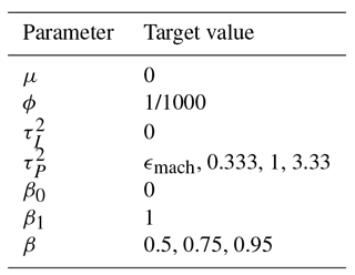
The parameter values prescribed for the target data are listed in Table C2. The instrumental observations are identical to the true target values, and the instrumental error variance $τ_{I}^{2}$ is therefore zero. The proxy noise variance $τ_{P}^{2}$ is varied systematically for the different SNR through the relation in Eq. (12).

The mean of the posterior distributions of the BARCAST parameters $α, μ, σ^{2}, 1 / ϕ$ , $τ_{I}^{2}$ and β₀ are listed in Table C3, together with the reconstructed SNR.

Table C1List of parameters defined in BARCAST, form of prior and hyperparameters.

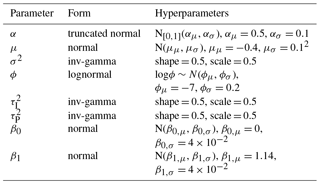
Download Print Version | Download XLSX

Table C2List of parameter values defined for the target data set. The four values of $τ_{P}^{2}$ listed are related to the four different signal-to-noise ratios: $SNR = \frac{1}{τ_{P}^{2}}$ . ϵ_mach is machine epsilon, the smallest positive number represented by the computer.

Download Print Version | Download XLSX

Table C3Mean of posterior distribution for each parameter.

Download Print Version | Download XLSX

Competing interests

The authors declare that they have no conflict of interest.

Acknowledgements

Tine Nilsen was supported by the Norwegian Research Council (KLIMAFORSK programme) under grant no. 229754, and partly by Tromsø Research Foundation via the UiT project A31054. Dmitry V. Divine was partly supported by Tromsø Research Foundation via the UiT project A33020. Johannes P. Werner gratefully acknowledges support from the Centre for Climate Dynamics (SKD) at the Bjerknes Centre. Dmitry V. Divine, Tine Nilsen and Johannes P. Werner also acknowledge the IS-DAAD project 255778 HOLCLIM for providing travel support. The authors would like to thank Kristoffer Rypdal for helpful discussions and comments.

Edited by: Jürg Luterbacher
Reviewed by: three anonymous referees

References

Beran, J., Feng, Y., Ghosh, S., and Kulik, R.: Long-Memory Processes, Springer, New York, 884 pp., 2013. a

Briffa, K. R., Jones, P. D., Bartholin, T. S., Eckstein, D., Schweingruber, F. H., Karlén, W., Zetterberg, P., and Eronen, M.: Fennoscandian summers from ad 500: temperature changes on short and long timescales, Clim. Dynam., 7, 111–119, https://doi.org/10.1007/BF00211153, 1992. a

Briffa, K. R., Osborn, T., Schweingruber, F. H., Harris, I. C., Jones, P. D., Shiyatov, S. G., and Vaganov, E.: Low frequency temperature variations from a northern tree ring density network, J. Geophys. Res.-Atmos., 106, 2929–2941, https://doi.org/10.1029/2000JD900617, 2001. a

Christiansen, B.: Reconstructing the NH Mean Temperature: Can Underestimation of Trends and Variability Be Avoided?, J. Climate, 24, 674–692, https://doi.org/10.1175/2010JCLI3646.1, 2011. a, b

Christiansen, B. and Ljungqvist, F. C.: Challenges and perspectives for large-scale temperature reconstructions of the past two millennia, Rev. Geophys., 55, 40–96, https://doi.org/10.1002/2016RG000521, 2017. a

Cook, E. R., Briffa, K. R., Meko, D. M., Graybill, D. A., and Funkhouser, G.: The 'segment length curse' in long tree-ring chronology development for palaeoclimatic studies, Holocene, 5, 229–237, https://doi.org/10.1177/095968369500500211, 1995. a, b

Dee, S., Parsons, L., Loope, G., Overpeck, J., Ault, T., and Emile-Geay, J.: Improved spectral comparisons of paleoclimate models and observations via proxy system modeling: Implications for multi-decadal variability, Earth Planet. Sc. Lett., 476, 34–46, https://doi.org/10.1016/j.epsl.2017.07.036, 2017. a

Dolman, A. M. and Laepple, T.: Sedproxy: a forward model for sediment archived climate proxies, Clim. Past Discuss., https://doi.org/10.5194/cp-2018-13, in review, 2018. a

Emile-Geay, J. and Tingley, M.: Inferring climate variability from nonlinear proxies: application to palaeo-ENSO studies, Clim. Past, 12, 31–50, https://doi.org/10.5194/cp-12-31-2016, 2016. a

Fraedrich, K. and Blender, R.: Scaling of Atmosphere and Ocean Temperature Correlations in Observations and Climate Models, Phys. Rev. Lett., 90, 108501, https://doi.org/10.1103/PhysRevLett.90.108501, 2003. a

Franke, J., Frank, D., Raible, C. C., Esper, J., and Bronnimann, S.: Spectral biases in tree-ring climate proxies, Nat. Clim. Change, 3, 360–364, https://doi.org/10.1038/NCLIMATE1816, 2013. a, b, c

Franzke, C. L. E., Graves, T., Watkins, N. W., Gramacy, R. B., and Hughes, C.: Robustness of estimators of long-range dependence and self-similarity under non-Gaussianity, Philo. T. Roy. Soc. A, 370, 1250–1267, https://doi.org/10.1098/rsta.2011.0349, 2012. a

Fredriksen, H.-B. and Rypdal, K.: Spectral Characteristics of Instrumental and Climate Model Surface Temperatures, J. Climate, 29, 1253–1268, https://doi.org/10.1175/JCLI-D-15-0457.1, 2016. a, b, c, d

Fredriksen, H.-B. and Rypdal, M.: Long-Range Persistence in Global Surface Temperatures Explained by Linear Multibox Energy Balance Models, J. Climate, 30, 7157–7168, https://doi.org/10.1175/JCLI-D-16-0877.1, 2017. a

Gelman, A., Carlin, J., Stern, H., and Rubin, D.: Bayesian Data Analysis, 2nd ed., Chapman & Hall, New York, 668 pp., 2003. a, b

Gneiting, T. and Raftery, A. E.: Strictly Proper Scoring Rules, Prediction, and Estimation, J. Am. Stat. Assoc., 102, 359–378, https://doi.org/10.1198/016214506000001437, 2007. a, b, c, d

Gómez-Navarro, J. J., Werner, J., Wagner, S., Luterbacher, J., and Zorita, E.: Establishing the skill of climate field reconstruction techniques for precipitation with pseudoproxy experiments, Clim. Dynam., 45, 1395–1413, 2015. a

Hasselmann, K.: Stochastic climate models Part I. Theory, Tellus, 28, 473–485, https://doi.org/10.1111/j.2153-3490.1976.tb00696.x, 1976. a

Helama, S., Melvin, T. M., and Briffa, K. R.: Regional curve standardization: State of the art, Holocene, 27, 172–177, https://doi.org/10.1177/0959683616652709, 2017. a

Hersbach, H.: Decomposition of the Continuous Ranked Probability Score for Ensemble Prediction Systems, Weather Forecast., 15, 559–570, https://doi.org/10.1175/1520-0434(2000)015<0559:DOTCRP>2.0.CO;2, 2000. a, b

Huybers, P. and Curry, W.: Links between annual, Milankovitch and continuum temperature variability, Nature, 441, 329–332, https://doi.org/10.1038/nature04745, 2006. a, b

Jones, P. D., Briffa, K. R., Barnett, T. P., and Tett, S. F. B.: High-resolution palaeoclimatic records for the last millennium: interpretation, integration and comparison with General Circulation Model control-run temperatures, Holocene, 8, 455–471, https://doi.org/10.1191/095968398667194956, 1998. a

Koscielny-Bunde, A. B., Havlin, S., and Goldreich, Y.: Analysis of daily temperature fluctuations, Physica A, 231, 393–396, https://doi.org/10.1016/0378-4371(96)00187-2, 1996. a

Lee, T. C. K., Zwiers, F. W., and Tsao, M.: Evaluation of proxy-based millennial reconstruction methods, Clim. Dynam., 31, 263–281, https://doi.org/10.1007/s00382-007-0351-9, 2008. a

Lovejoy, S. and Schertzer, D.: Low Frequency Weather and the Emergence of the Climate, 231–254, 196, American Geophysical Union, https://doi.org/10.1029/2011GM001087, 2012. a

Luterbacher, J., Werner, J. P., Smerdon, J. E., Fernández-Donado, L., González-Rouco, F. J., Barriopedro, D., Ljungqvist, F. C., Büntgen, U., Zorita, E., Wagner, S., Esper, J., McCarroll, D., Toreti, A., Frank, D., Jungclaus, J. H., Barriendos, M., Bertolin, C., Bothe, O., Brázdil, R., Camuffo, D., Dobrovolný, P., Gagen, M., García-Bustamante, E., Ge, Q., Gómez-Navarro, J. J., Guiot, J., Hao, Z., Hegerl, G. C., Holmgren, K., Klimenko, V. V., Martín-Chivelet, J., Pfister, C., Roberts, N., Schindler, A., Schurer, A., Solomina, O., von Gunten, L., Wahl, E., Wanner, H., Wetter, O., Xoplaki, E., Yuan, N., Zanchettin, D., Zhang, H., and Zerefos, C.: European summer temperatures since Roman times, Environ. Res. Lett., 11, 024001, https://doi.org/10.1088/1748-9326/11/2/024001, 2016. a, b

Malamud, B. D. and Turcotte, D. L.: Self-affine time series: measures of weak and strong persistence, J. Stat. Plan. Infer., 80, 173–196, https://doi.org/10.1016/S0378-3758(98)00249-3, 1999. a, b

Mann, M. E., Bradley, R. S., and Hughes, M. K.: Global-scale temperature patterns and climate forcing over the past six centuries, Nature, 392, 779–787, 1998. a

Mann, M. E., Rutherford, S., Wahl, E., and Ammann, C.: Testing the Fidelity of Methods Used in Proxy-Based Reconstructions of Past Climate, J. Climate, 18, 4097–4107, https://doi.org/10.1175/JCLI3564.1, 2005. a

Mann, M. E., Rutherford, S., Wahl, E., and Ammann, C.: Robustness of proxy-based climate field reconstruction methods, J. Geophys. Res., 112, D12109, https://doi.org/10.1029/2006JD008272, 2007. a, b

Mann, M. E., Zhang, Z., Hughes, M. K., Bradley, R. S., Miller, S. K., Rutherford, S., and Ni, F.: Proxy-based reconstructions of hemispheric and global surface temperature variations over the past two millennia, P. Natl. Acad. Sci. USA, 105, 13252–13257, https://doi.org/10.1073/pnas.0805721105, 2008. a, b

Mann, M. E., Zhang, Z., Rutherford, S., Bradley, R. S., Hughes, M. K., Shindell, D., Ammann, C., Faluvegi, G., and Ni, F.: Global Signatures and Dynamical Origins of the Little Ice Age and Medieval Climate Anomaly, Science, 326, 1256–1260, 2009. a, b

Melvin, T. M. and Briffa, K. R.: A signal-free approach to dendroclimatic standardisation, Dendrochronologia, 26, 71–86, https://doi.org/10.1016/j.dendro.2007.12.001, 2008. a

Moberg, A., Sonechkin, D. M., Holmgren, K., Datsenko, N. M., and Karlén, W.: Highly variable Northern Hemisphere temperatures reconstructed from low-and high-resolution proxy data, Nature, 433, 613–617, https://doi.org/10.1038/nature03265, 2005. a

Nilsen, T., Rypdal, K., and Fredriksen, H.-B.: Are there multiple scaling regimes in Holocene temperature records?, Earth Syst. Dynam., 7, 419–439, https://doi.org/10.5194/esd-7-419-2016, 2016. a, b, c, d

North, G. R., Wang, J., and Genton, M. G.: Correlation models for temperature fields, J. Climate, 24, 5850–5862, https://doi.org/10.1175/2011JCLI4199.1, 2011. a, b, c

PAGES 2k Consortium: Continental-scale temperature variability during the past two millennia, Nat. Geosci., 6, 339–346, https://doi.org/10.1038/ngeo1797, 2013. a

Peng, C.-K., Buldyrev, S. V., Havlin, S., Simons, M., Stanley, H. E., and Goldberger, A. L.: Mosaic organization of DNA, Phys. Rev. E, 49, 1685–1689, https://doi.org/10.1103/PhysRevE.49.1685, 1994. a

Rybski, D., Bunde, A., Havlin, S., and von Storch, H.: Long-term persistence in climate and the detection problem, Geophys. Res. Lett., 33, L06718, https://doi.org/10.1029/2005GL025591, 2006. a, b

Rypdal, M. and Rypdal, K.: Long-memory effects in linear-response models of Earth's temperature and implications for future global warming, J. Climate, 27, 5240–5258, https://doi.org/10.1175/JCLI-D-13-00296.1, 2014. a

Rypdal, M. and Rypdal, K.: Late Quaternary temperature variability described as abrupt transitions on a 1/f noise background, Earth Syst. Dynam., 7, 281–293, https://doi.org/10.5194/esd-7-281-2016, 2016. a, b

Rypdal, K., Østvand, L., and Rypdal, M.: Long-range memory in Earth's surface temperature on time scales from months to centuries, J. Geophys. Res., 118, 7046–7062, https://doi.org/10.1002/jgrd.50399, 2013. a, b

Rypdal, K., Rypdal, M., and Fredriksen., H. B.: Spatiotemporal Long-Range Persistence in Earth's Temperature Field: Analysis of Stochastic-Diffusive Energy Balance Models, J. Climate, 28, 8379–8395, https://doi.org/10.1175/JCLI-D-15-0183.1, 2015. a, b

Schneider, T.: Analysis of Incomplete Climate Data: Estimation of Mean Values and Covariance Matrices and Imputation of Missing Values, J. Climate, 14, 853–871, https://doi.org/10.1175/1520-0442(2001)014<0853:AOICDE>2.0.CO;2, 2001. a

Smerdon, J. E.: Climate models as a test bed for climate reconstruction methods: pseudoproxy experiments, Wiley Interdisciplinary Reviews: Climate Change, 3, 63–77, https://doi.org/10.1002/wcc.149, 2012. a, b, c, d

Smerdon, J. E., Kaplan, A., Zorita, E., González-Rouco, J. F., and Evans, M. N.: Spatial performance of four climate field reconstruction methods targeting the Common Era, Geophys. Res. Lett., 38, L11705, https://doi.org/10.1029/2011GL047372, l11705, 2011. a

Tingley, M. P. and Huybers, P.: A Bayesian Algorithm for Reconstructing Climate Anomalies in Space and Time. Part 1: Development and Applications to Paleoclimate Reconstruction Problems, J. Climate, 23, 2759–2781, https://doi.org/10.1175/2009JCLI3015.1, 2010a. a, b, c, d, e

Tingley, M. P. and Huybers, P.: A Bayesian Algorithm for Reconstructing Climate Anomalies in Space and Time. Part II: Comparison with the Regularized Expectation-Maximization Algorithm, J. Climate, 23, 2782–2800, https://doi.org/10.1175/2009JCLI3016.1, 2010b. a, b

Tingley, M. P. and Li, B.: Comments on ”Reconstructing the NH Mean Temperature: Can Underestimation of Trends and Variability Be Avoided?, J. Climate, 25, 3441–3446, https://doi.org/10.1175/JCLI-D-11-00005.1, 2012. a

Tipton, J., Hooten, M., Pederson, N., Tingley, M., and Bishop, D.: Reconstruction of late Holocene climate based on tree growth and mechanistic hierarchical models, Environmetrics, 27, 42–54, https://doi.org/10.1002/env.2368, 2015. a, b

Wahl, E. R., Diaz, H. F., Vose, R. S., and Gross, W. S.: Multicentury Evaluation of Recovery from Strong Precipitation Deficits in California, J. Climate, 30, 6053–6063, https://doi.org/10.1175/JCLI-D-16-0423.1, 2017. a, b

Wang, J., Emile-Geay, J., Guillot, D., Smerdon, J. E., and Rajaratnam, B.: Evaluating climate field reconstruction techniques using improved emulations of real-world conditions, Clim. Past, 10, 1–19, https://doi.org/10.5194/cp-10-1-2014, 2014. a, b, c

Wang, J., Emile-Geay, J., Guillot, D., McKay, N. P., and Rajaratnam, B.: Fragility of reconstructed temperature patterns over the Common Era: Implications for model evaluation, Geophys. Res. Lett., 42, 7162–7170, https://doi.org/10.1002/2015GL065265, 2015. a

Werner, J. P. and Tingley, M. P.: Technical Note: Probabilistically constraining proxy age-depth models within a Bayesian hierarchical reconstruction model, Clim. Past, 11, 533–545, https://doi.org/10.5194/cp-11-533-2015, 2015. a, b, c, d

Werner, J. P., Luterbacher, J., and Smerdon, J. E.: A Pseudoproxy Evaluation of Bayesian Hierarchical Modeling and Canonical Correlation Analysis for Climate Field Reconstructions over Europe, J. Climate, 26, 851–867, https://doi.org/10.1175/JCLI-D-12-00016.1, 2013. a, b, c, d, e, f, g

Werner, J. P., Toreti, A., and Luterbacher, J.: Stochastic models for climate reconstructions – how wrong is too wrong?, in: NOLTA2014 (2014 International Symposium on Nonlinear Theory and its Applications), 2014. a, b

Werner, J. P., Divine, D. V., Charpentier Ljungqvist, F., Nilsen, T., and Francus, P.: Spatio-temporal variability of Arctic summer temperatures over the past 2 millennia, Clim. Past, 14, 527–557, https://doi.org/10.5194/cp-14-527-2018, 2018. a, b, c, d, e, f, g

Wonnacott, R. J. and Wonnacott, T. H.: Econometrics, Probability and Mathematical Statistics, John Wiley and Sons, New York, 604 pp., 1979. a

Zhang, H., Yuan, N., Esper, J., Werner, J. P., Xoplaki, E., Büntgen, U., Treydte, K., and Luterbacher, J.: Modified climate with long term memory in tree ring proxies, Environ. Res. Lett., 10, 084020, https://doi.org/10.1088/1748-9326/10/8/084020, 2015. a, b

Zhang, H., Werner, J. P., Garćia-Bustamante, E., Gonźalez-Rouco, F., Wagner, S., Zorita, E., Fraedrich, K., Jungclaus, J. H., Ljungqvist, F. C., Zhu, X., Xoplaki, E., Chen, F., Duan, J., Ge, Q., Hao, Z., Ivanov, M., Schneider, L., Talento, S., Wang, J., Yang, B., and Luterbacher, J.: East Asian warm season temperature variations over the past two millennia, Sci. Rep.-UK, 8, 7702, https://doi.org/10.1038/s41598-018-26038-8, 2018. a

Articles

Short summary

The BARCAST climate field reconstruction method is tested using synthetic data experiments. It is demonstrated that the output reconstructions have altered statistical properties compared with the input data, but they are also not necessarily consistent with the model assumption of the reconstruction method. The conclusion is that the statistical properties of a reconstruction not only reflect the statistics of the real climate, but they may very well be affected by the manipulation of the data.