the Creative Commons Attribution 4.0 License.
the Creative Commons Attribution 4.0 License.
 | 02 Jul 2019
Role of the stratospheric chemistry–climate interactions in the hot climate conditions of the Eocene
Rémi Thiéblemont
Slimane Bekki
Svetlana Botsyun
Pierre Sepulchre
The stratospheric ozone layer plays a key role in atmospheric thermal structure and circulation. Although stratospheric ozone distribution is sensitive to changes in trace gases concentrations and climate, the modifications of stratospheric ozone are not usually considered in climate studies at geological timescales. Here, we evaluate the potential role of stratospheric ozone chemistry in the case of the Eocene hot conditions. Using a chemistry–climate model, we show that the structure of the ozone layer is significantly different under these conditions (4×CO2 climate and high concentrations of tropospheric N2O and CH4). The total column ozone (TCO) remains more or less unchanged in the tropics whereas it is found to be enhanced at mid- and high latitudes. These ozone changes are related to the stratospheric cooling and an acceleration of stratospheric Brewer–Dobson circulation simulated under Eocene climate. As a consequence, the meridional distribution of the TCO appears to be modified, showing particularly pronounced midlatitude maxima and a steeper negative poleward gradient from these maxima. These anomalies are consistent with changes in the seasonal evolution of the polar vortex during winter, especially in the Northern Hemisphere, found to be mainly driven by seasonal changes in planetary wave activity and stratospheric wave-drag. Compared to a preindustrial atmospheric composition, the changes in local ozone concentration reach up to 40 % for zonal annual mean and affect temperature by a few kelvins in the middle stratosphere.
As inter-model differences in simulating deep-past temperatures are quite high, the consideration of atmospheric chemistry, which is computationally demanding in Earth system models, may seem superfluous. However, our results suggest that using stratospheric ozone calculated by the model (and hence more physically consistent with Eocene conditions) instead of the commonly specified preindustrial ozone distribution could change the simulated global surface air temperature by as much as 14 %. This error is of the same order as the effect of non-CO2 boundary conditions (topography, bathymetry, solar constant and vegetation). Moreover, the results highlight the sensitivity of stratospheric ozone to hot climate conditions. Since the climate sensitivity to stratospheric ozone feedback largely differs between models, it must be better constrained not only for deep-past conditions but also for future climates.
Please read the corrigendum first before continuing.
-
Notice on corrigendum
The requested paper has a corresponding corrigendum published. Please read the corrigendum first before downloading the article.
-
Article
(3195 KB)
- Corrigendum
-
Supplement
(433 KB)
-
The requested paper has a corresponding corrigendum published. Please read the corrigendum first before downloading the article.
- Article
(3195 KB) - Corrigendum
-
Supplement
(433 KB) - BibTeX
- EndNote


The absorption of incoming solar ultraviolet (UV) radiation by stratospheric ozone is responsible for the heating up of the stratosphere and hence its dynamical stability. In addition, this absorption is essential to the development of life because it prevents this very harmful UV radiation from reaching the Earth's surface. Stratospheric ozone is thus a key component of the radiative equilibrium and habitability of the Earth (Brasseur and Solomon, 2005). However, although deep-time climates are more and more investigated with numerical climate models, the role of the stratosphere in such climates is usually neglected (e.g., Kageyama et al., 2017; Lunt et al., 2017).
The present-day stratosphere has been intensively studied to understand, anticipate and mitigate the global ozone depletion caused by the emissions of anthropogenic halogenated compounds such as chlorofluorocarbons and halons in the second part of the 20th century (WMO, 2014). The phasing out of the emissions has led to the start of a stratospheric ozone recovery since the end of the 1990s (Chipperfield et al., 2017). However, in the context of increasing levels of greenhouse gases (GHGs, e.g., CO2, N2O and CH4) and associated climate change, the sensitivity of stratospheric ozone to other drivers, especially climate-related drivers, is increasingly investigated. For example, stratospheric ozone is sensitive to changes in N2O, CH4 and water vapor levels. N2O enters in the stratosphere at the tropical tropopause and controls the levels of NOx, which are the most efficient ozone-destroying radicals in the middle stratosphere. Enhanced CH4 levels increase ozone production in the troposphere and lower stratosphere but also lead to higher water vapor levels, which tend to favor ozone destruction (Bekki et al., 2011; Revell et al., 2012). An increase in CO2 concentration results in a cooling of the stratosphere, which slows down ozone destruction in the upper stratosphere and hence favors ozone recovery in this region. In addition to stratospheric chemical changes, the ongoing climate change tends to intensify the large-scale stratospheric overturning circulation (the so-called Brewer–Dobson circulation), which is responsible for upward transport of air in the tropics and poleward and downward transport at middle and high latitudes (see, e.g., Butchart, 2014, and references therein). These circulation changes result in reduced ozone levels in the tropical lower stratosphere due to the faster ascent of air in the lower tropical stratosphere (Avallone and Prather, 1996) and enhanced ozone levels at middle and high latitudes (Bekki et al., 2011). This illustrates how stratospheric ozone responds to climate change. More recently, Chiodo et al. (2018) presented an analysis of the stratospheric ozone layer response to an abrupt quadrupling of CO2 concentration in four chemistry climate models. As found previously (see, e.g., WMO, 2014), they showed that increased CO2 levels in the four models lead to a decrease in ozone concentration in the tropical lower stratosphere and an increase at high latitudes and in the upper stratosphere. However, there were large differences between models in the magnitude of the ozone response.
At the same time, stratospheric ozone changes also influence the climate. For instance, climate models have to account for the formation of the stratospheric ozone hole to be able to reproduce correctly the trends in Antarctic surface temperatures observed during the last half century (e.g., Son et al., 2010; McLandress et al., 2011). Considering larger climate perturbations, Nowack et al. (2015) performed an abrupt 4×CO2 experiment with a comprehensive ocean–atmosphere–chemistry–climate model and found that neglecting stratospheric ozone changes triggered by CO2 increase (i.e., specifying a fixed ozone climatology in the model) led to the overestimation of the surface global mean temperature response by about 1 K (i.e., 20 % of the total surface temperature response). Chiodo and Polvani (2017) carried out the same numerical experiment (4×CO2) with a different chemistry–climate model and found that, in contrast to the Nowack et al. (2015) results, stratospheric ozone changes played a negligible role in the global surface temperature response. Nonetheless, they found that the stratospheric ozone feedback in their model significantly reduced the CO2-induced poleward shift of the midlatitude tropospheric jet by lowering the strength of the meridional temperature gradient near the tropopause. These results suggest that stratospheric ozone perturbations should be accounted for in climate models in order to fully capture the climate response to GHG changes.
In the past of the Earth, the oxygenated atmosphere has encountered hot climatic conditions due to strong greenhouse effects. During the early Eocene (∼56–50 Ma) terrestrial temperatures at high latitudes were possibly up to 20 K higher than modern ones (Masson-Delmotte et al., 2013). Under such a warm climate, biogenic emissions of N2O and CH4 were likely to be drastically boosted, being 4 to 5 times higher than the preindustrial ones (Beerling et al., 2011). Note, however, that, in most modeling studies of deep-time climates, the role of non-CO2 gases is neglected (e.g., DeepMIP; Lunt et al., 2017). Beerling et al. (2011) studied the tropospheric chemical composition under a warm climate and potentially high biogenic emissions of the early Eocene (55 Ma). Using an Earth system model including tropospheric chemistry, they found that the OH concentration, which is the main oxidant for most compounds in the troposphere, was significantly reduced (by 14 % to 50 %) due to higher levels of compounds to oxidize. The high tropospheric levels of reactive greenhouse gases (N2O, CH4 and O3) were maintained under these conditions. Considering the full Earth system interactions, and in particular albedo change due to the melting of continental snow, Beerling et al. (2011) calculated an increase of 1.4 to 2.7 K in surface temperatures due to tropospheric chemical composition changes for the Eocene. However, since their model did not include stratospheric chemistry, they could not study stratospheric composition changes. Unger and Yue (2014) investigated the chemistry–climate feedbacks in the mid-Pliocene (∼3 Ma) using a vegetation–chemistry–climate model simulating both stratospheric and tropospheric chemistry. This epoch is cooler than the Eocene but still of interest because its global climate is thought to be as warm as the climate projected for the end of the ongoing century (+2–3 K compared to the present day). Compared to preindustrial conditions (PI), the Unger and Yue (2014) model simulations indicated that the mid-Pliocene ozone burden was higher by 25 % in the troposphere and by 5 % in the stratosphere. The global stratospheric ozone increase, resulting from a stronger tropical upwelling and less ozone destruction in the stratosphere, led to a 20 % decrease in tropospheric ozone photolysis and hence OH production. As a consequence, tropospheric OH concentrations were reduced by 20 %–25 % and hence the lifetime and burden of important reactive species (CO, CH4) were significantly increased. Unger and Yue (2014) showed that the warming effect of the changes in chemically reactive compounds (i.e., CH4, N2O, tropospheric O3) could have represented ∼75 % of the warming from CO2 increase. The studies of Beerling et al. (2011) and Unger and Yue (2014) suggest that non-CO2 greenhouse gases may have played a significant role in the overall climate in the Cenozoic greenhouse worlds.
As pointed out previously, most studies of Cenozoic paleoclimates assume that the atmospheric composition is fixed except for CO2 because there is no estimate of these composition changes. The purpose of this paper is (i) to investigate, using a stratospheric chemistry–climate model, to what extent the stratosphere, notably the ozone layer, might have been different in the early Eocene conditions and (ii) to estimate the possible effects of these stratospheric changes on the tropospheric oxidizing capacity and climate. The Eocene is characterized by high surface temperatures, elevated CO2 levels, the absence of ice caps and a large extent of tropical vegetation. High CH4 and N2O levels are also expected based on Earth system model (ESM) simulations (Beerling et al., 2011). Whereas the data are sparse and have large uncertainties for the geological past, several proxy-based reconstructions of CO2 levels and surface temperatures have been released. They have notably been used to build a harmonized protocol for climate modeling of the early Eocene (Lunt et al., 2017), which will be used to intercompare climate model sensitivity during the ongoing Paleoclimate Modelling Intercomparison Project (PMIP4). This protocol gathers recommendations on paleogeography, land cover, CO2 and CH4 concentrations, natural aerosols, solar constant, and astronomical parameters, but no recommendations have been provided yet for stratospheric conditions. In this work, we propose to examine the role of the stratospheric ozone layer in Eocene climate. We first investigate the stratospheric ozone response to GHG-induced warm climate such as the one expected under Eocene conditions and compare it to preindustrial climate conditions. We then discuss the methodology to account properly for these stratospheric ozone changes in deep-time paleoclimate simulations. Finally, based on the model simulations, we estimate the difference in UV radiation reaching the Earth surface between this epoch and the preindustrial period and the resulting impact on tropospheric chemistry. The potential climate forcing of the stratospheric changes is also discussed.
2.1 The LMDz–REPROBUS climate–chemistry model
Simulations are performed with the stratospheric chemistry–climate model developed in the framework of the IPSL Earth system model (IPSL-CM, climate model) development (Dufresne et al., 2013). The stratospheric chemistry is computed with the REPROBUS chemical model (Lefèvre et al., 1994, 1998; Jourdain et al., 2008) coupled with the LMDz atmospheric general circulation model (Hourdin et al., 2013). REPROBUS describes the chemistry of stratospheric source gases such as N2O, CH4, CH3Cl and CH3Br and the associated radical chemistry of hydrogen, nitrogen oxides, chlorine and bromine species. It computes the global distribution of trace gases, aerosols and clouds within the stratosphere considering gas-phase and heterogeneous chemistry. The heterogeneous chemistry component takes into account the reactions on sulfuric acid aerosols and liquid (ternary solution) and solid (nitric acid trihydrate particles, ice) polar stratospheric clouds (PSCs). The gravitational sedimentation of PSCs is simulated as well. The LMDz–REPROBUS chemistry–climate model allows an interactive coupling of ozone, shortwave heating rates and dynamics as recommended in Sassi et al. (2005). The resolution of the model is 3.75∘ in longitude and 1.9∘ in latitude, and it has 39 vertical levels, with around 15 levels above 20 km and around 24 above 10 km and a lid height at ∼70 km.
LMDz and LMDz–REPROBUS have been involved in a large range of studies, model intercomparisons and evaluations, notably through the participation of the LMDz model in the international Coupled Model Intercomparison Project (CMIP, phases 3, 5 and currently 6) and the participation of LMDz–REPROBUS in the Chemistry Climate Model Validation (SPARC CCMVal, 2010) and the Chemistry Climate Model Initiative (CCMI; Morgenstern et al., 2017). Results presented in the recent studies of, e.g., de la Cámara et al. (2016a, b), Thiéblemont et al. (2017) and Ayarzagüena et al. (2018) have shown that the stratospheric chemistry, dynamics and transport simulated by the LMDz model and its chemistry–climate model version are consistent with satellite observations, reanalysis and other models of the same kind.
2.2 Simulation setup
The setup of the four simulations performed in this study is summarized in Table 1. All the simulations consist of 30-year time slices, starting from atmospheric physical conditions and surface temperatures taken from very long coupled atmosphere–ocean simulations. For the analysis of our chemistry–climate simulations, a 5-year spin-up is considered. For all the simulations, the solar constant is set to 1366 W m−2 and orbital parameters (obliquity, precession and eccentricity) are set to modern values as recommended in the DeepMIP protocol (model intercomparison project; Lunt et al., 2017). Oxygen variations are poorly constrained over pre-Quaternary timescales, and there is no consensus on the oxygen variations through the Cenozoic (see Fig. 1 of Wade et al., 2018). In view of these uncertainties, we use a present-day oxygen content to investigate Cenozoic past climates, as commonly done in climate models.
Table 1Setup of LMDz. AMIP is the Atmospheric Model Intercomparison Project.
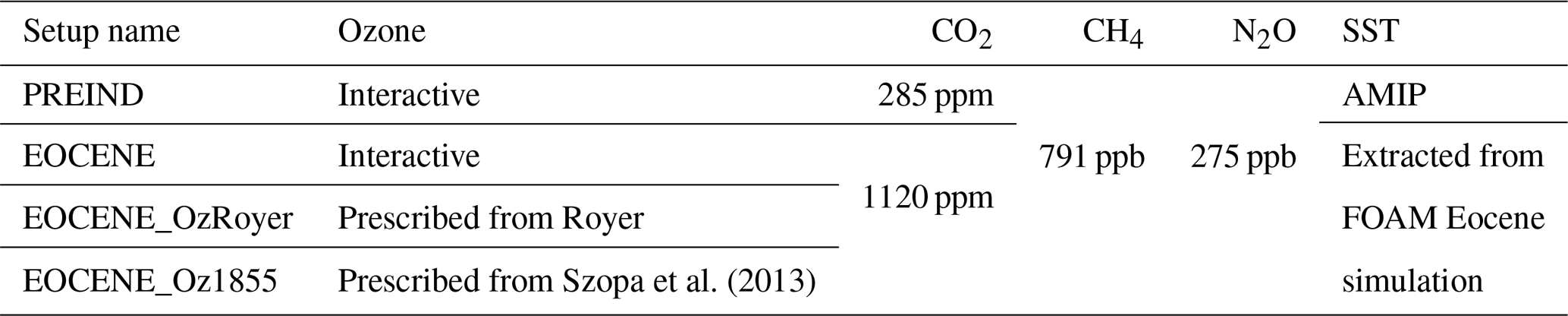
Note: for the Eocene simulations, the REPROBUS chemical model considers a CH4 concentration of 3614 ppb and an N2O concentration of 323 ppb.

2.2.1 Preindustrial simulations
The boundary conditions of our preindustrial experiment (PREIND) include modern topography, a land–sea mask, ice sheets and climatological mean values computed over the 1870–1899 period for sea surface temperatures (SSTs) and sea-ice extent. Greenhouse gases are set to preindustrial values, i.e., a CO2 level at 285 ppm, a CH4 level at 791 ppb and an N2O level at 275 ppb. Halogenated ozone-depleting substances of anthropogenic origin (i.e., fluorocarbons) are set to zero. Naturally emitted halogenated compounds (CH3Br and CH3Cl) are prescribed at their preindustrial levels (respectively, 7 and 482 ppb).
2.2.2 Eocene base case simulation
As for the PREIND experiment, the Eocene experiment (EOCENE) includes interactive chemistry, which allows us to calculate stratospheric composition. The physical boundary conditions for the EOCENE experiment (e.g., SSTs, sea ice, land surface properties) are based on a climate simulation done with the fully coupled low-resolution Fast Ocean Atmosphere Model (FOAM; Jacob, 1997) and the Lund–Potsdam–Jena (LPJ) dynamic global vegetation model (Sitch et al., 2003) coupled offline as illustrated Fig. 1. The LPJ–FOAM coupled ocean–atmosphere–vegetation simulation provides the surface conditions (SSTs, land surface conditions) required to simulate the climate with the LMDz atmospheric general circulation model. FOAM is forced with the Eocene paleogeography reconstruction of Herold et al. (2014). Compared to the present-day paleogeography, it includes major modifications, namely closed Drake and Tasman seaways, an open Central American Seaway, and an open Paratethys Sea. Topography is altered as well, with a lower Tibetan Plateau and Andes. CO2 is set to 1120 ppm, equivalent to a 4×CO2 preindustrial level ([CO2]PI), as Eocene CO2 estimates range between 400 and 2400 ppm (as reported by Lunt et al., 2017, based on boron isotopes analysis from Anagostou et al., 2016). This CO2 value lies at the low end of the Eocene-compatible GHG forcing ranges, in particular those recommended by the DeepMIP project, which proposes to test 3×[CO2]PI, 6×[CO2]PI and 12×[CO2]PI (Lunt et al., 2017). After 2000 model years, SSTs simulated by FOAM are averaged over the last 100-year period to build a 12-month (seasonally varying) climatology used as a boundary condition for LMDz. FOAM coupling with the LPJ vegetation model provides equilibrated vegetation as well, whose albedo and rugosity are extracted to serve as continental boundary conditions for LMDz. The global mean SST that we use are 17.3 ∘C for the preindustrial period and 23.9 ∘C for the Eocene. These values lie in the ranges presented for four model realizations in Lunt et al. (2012). These ranges are between 15.2 and 17.9 ∘C for PI and between 22.2 and 26.4 ∘C for the Eocene when considering 4×[CO2]PI (Note that when CO2 varies from 2×[CO2]PI to 16×[CO2]PI, the range of SST is between 21.4 and 29.7 ∘C; Lunt et al., 2012.) In addition, the meridional surface temperature gradient is 24.6 ∘C over ocean and 33.7 ∘C over land in our protocol when the ranges with the 4×[CO2]PI experiments shown in Lunt et al. (2012) are [24; 33] ∘C and [25.5; 37] ∘C, respectively. Numerous recently published paleoclimate studies are based on the two-step methodology based on FOAM-LPJ and LMDz, and this setup has been shown to perform well (e.g., Ladant et al., 2014; Licht et al., 2014; Ladant and Donnadieu, 2016; Pohl et al., 2016; Porada et al., 2016; Botsyun et al., 2019).
Applying a coupled vegetation–atmosphere to the particularly warm climate of the early Eocene (55 Ma), Beerling et al. (2011) have estimated that CH4 and N2O concentrations should have been much higher than nowadays and could have lain in the 2384–3614 and 323–426 ppb ranges, respectively. The direct climate impact of highly enhanced CH4 and N2O levels is accounted for by setting CO2 to a high level (1120 ppm) in the radiative module in our atmospheric circulation model (Table 1). Ozone chemistry is affected by changes in N2O and CH4 (e.g., Revell et al., 2012). To account for this effect, there are CH4 and N2O chemically active tracers in the REPROBUS chemical model (i.e., modified by the transport and chemistry schemes). Their surface concentrations are taken from the modeling study of Beerling et al. (2011), and CH4 and N2O surface concentrations are set to 3614 and 323 ppb, respectively, in the chemistry module (REPROBUS). Their global distributions change with time during a simulation, but they are not used as inputs to the radiative scheme and hence their changes do not affect the climate; only ozone changes do.
2.2.3 Eocene simulations with prescribed stratospheric ozone
In addition to the EOCENE experiment in which stratospheric ozone is calculated interactively, two other Eocene simulations (EOCENE_OzRoyer, EOCENE_Oz1855) are performed in which different climatological ozone representations are specified instead of ozone being calculated interactively. The ozone climatology in the EOCENE_OzRoyer experiment is rather typical of the 1980s ozone distribution. It originates from fits to the ozone profile from Krueger and Mintzner (1976) and variations with altitude and latitude of the maximum ozone concentrations and total column ozone from Keating and Young (1985). This OzRoyer ozone climatology was constructed by J.-F. Royer (CNRM, Meteo France) and implemented in the LMDz atmospheric circulation model in the 1980s. The Oz1855 ozone climatology in the EOCENE_Oz1855 experiment is more representative of the preindustrial period. It is based on an 11-year mean climatology centered on 1855 derived from historical transient LMDz–REPROBUS simulations (Szopa et al., 2013). This ozone climatology is commonly used for the simulation of past climates with the LMDz model.
The comparison between EOCENE and PREIND experiments, which both include the interactive chemistry of the stratosphere, allows us to explore and quantify the impacts of the Eocene warm climate on stratospheric circulation and composition (Sect. 3). Furthermore, comparing the EOCENE experiment with EOCENE_OzRoyer and EOCENE_Oz1855 experiments allows us to assess the role of the stratospheric ozone representation on the climate response to Eocene extreme conditions (Sect. 4). Note that the statistical significance of anomaly fields is estimated here using a Student's t test.
3.1 Stratospheric ozone in Eocene conditions
We first investigate the impact of Eocene conditions on stratospheric ozone with respect to preindustrial conditions. Figure 2a and b show the latitude vs. pressure zonally averaged cross sections of temperature and ozone anomalies associated with the Eocene conditions. As expected, the CO2 increase leads to a global radiative cooling of the stratosphere with decreases in temperatures exceeding 12 K above 10 hPa (∼32 km) and a warming of the troposphere (Fig. 2a). In the troposphere, we further notice a more pronounced Antarctic amplification of the temperature signals, which contrasts with present-day climate conditions where a more pronounced Arctic amplification of the global warming is observed (IPCC, 2013). This signal, consistently simulated by several models (Lunt et al., 2012), is linked to the absence of the Antarctic ice sheet in Eocene boundary conditions, which leads to lower surface topography and albedo. The cooling of the stratosphere slows down the ozone destruction, resulting in an increase in stratospheric ozone concentrations (Haigh and Pyle, 1982). This is consistent with the statistically significant positive ozone anomalies found above 50 hPa (∼20 km) over the polar regions and above 10 hPa in the tropical band (Fig. 2b). Note that this effect increases with altitude in the stratosphere as the photochemical control on ozone levels becomes prominent (Brasseur and Solomon, 2005). Similarly to the results of Chiodo et al. (2018), which investigate the effect of quadrupling CO2 by starting from preindustrial climate, a maximum ozone increase of ∼40 % is found at about 2–3 hPa (∼40 km). Note that in our simulation, the stratospheric chemistry is also modified by the increase in N2O and CH4. However, their effect only reaches a maximum of 3 % in the equatorial upper stratosphere (∼5 hPa) (see Fig. S1 in the Supplement). Although this chemical effect on ozone is statistically significant, its impact appears to be small compared to the upper stratosphere 40 % increase in ozone due to increasing CO2.
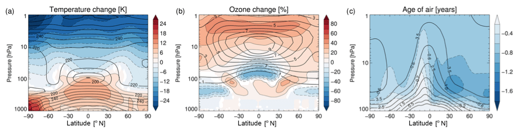
Figure 2Annual mean differences (EOCENE minus PREIND) of zonally averaged temperature (in K, a), ozone (in %, b) and age of air (in years, c). Color-filled contours in (a) and (b) indicate that anomalies are statistically different at the 1 % confidence level according to a t test. Black contours show the preindustrial climatology expressed in K (a), ppm (b) and years (c).
In contrast, the lower tropical stratosphere (30∘ S–30∘ N, 100–30 hPa) exhibits a statistically significant ozone decrease of up to 40 %. In this region, the ozone concentration is mostly controlled by transport processes (Brasseur and Solomon, 2005), especially the strength of the Brewer–Dobson circulation ascending branch. Figure 2c shows the age of air (AoA) calculated after 20 years of simulations by taking as a reference entry point the equatorial lowermost stratosphere, slightly above the tropopause (i.e., pressure level corresponding to 74 hPa). Globally, the stratospheric AoA is younger in the Eocene experiment than in the preindustrial one, revealing an acceleration of the Brewer–Dobson circulation under Eocene conditions. This, in turn, is consistent with the reduced ozone concentration in the lower tropical stratosphere. Note also that the tropopause height is globally lifted up in the Eocene experiment (not shown). The rise of the tropopause is a robust feature of warmer climate conditions (Sausen and Santer, 2003) and contributes to the negative ozone anomaly found in the vicinity of the tropopause region (Fig. 2b) (Dietmüller et al., 2014).
Next, we examine anomalies of the annual total column ozone (TCO). Figure 3 shows the comparison of the latitudinal distribution of the annual TCO for Eocene and preindustrial conditions. In both simulations (Fig. 3a), the TCO shows a minimum in the tropical region (20∘ S, 20∘ N) of ∼270 Dobson units (DU) and maxima near 55∘ N and 55∘ S, followed by poleward decreases that are more pronounced in the Southern Hemisphere. The differences between Eocene and preindustrial conditions (Fig. 3b) reveal no changes in the tropical band 20∘ S–20∘ N but statistically significant positive anomalies at midlatitudes and in polar regions. The midlatitude maxima reach ∼390 DU for preindustrial conditions, whereas they exceed 430 DU for Eocene conditions. This latitudinal distribution of TCO anomalies is overall consistent with projections of TCO anomalies simulated in response to the 21st-century climate change and post-CFC (chlorofluorocarbon) era (Li et al., 2009) or to an abrupt 4×CO2 increase from preindustrial climate conditions (Chiodo et al., 2018). The detailed comparison of our results with those of Chiodo et al. (2018) shows, however, noticeable differences at high latitudes. In our simulations, the TCO anomalies peak at 45∘ S and 50∘ N with maximum differences of 50 and 60 DU, respectively; the anomalies decrease from these maxima to about 30 DU at high latitudes (Fig. 3b). In Chiodo et al. (2018), hints of such a decrease were found in the Southern Hemisphere for only two out of the four models that are intercompared, and no such decrease was seen in the Northern Hemisphere. The negative poleward TCO gradient at high latitudes appears to strengthen markedly under Eocene conditions in the Northern Hemisphere (Fig. 3b). The seasonal dependence of the TCO high-latitude poleward gradient for the Eocene and preindustrial conditions in the Northern Hemisphere is explored in Fig. 4. Figure 4 reveals that, under Eocene conditions, the negative gradient is particularly pronounced during the winter season (from October to March), when the stratospheric polar vortex dominates the high-latitude circulation in the Northern Hemisphere. Hence, this indicates substantial changes in the stratospheric circulation associated with the Eocene conditions that we examine further in Sect. 3.2.
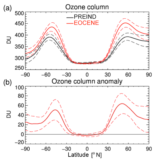
Figure 3Latitudinal profile of the total column ozone (in Dobson units or DU, a) in the (red) EOCENE and (black) PREIND simulation. Total column ozone change (in DU, b) between the EOCENE and PREIND simulation. Dashed lines delimit the 2σ uncertainty envelop, which is represented by the standard error of the mean.
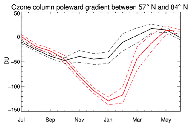
Figure 4Zonally averaged seasonal evolution of the latitudinal gradient (computed as the difference between 84 and 57∘ N) of the total column ozone for the EOCENE (red) and PREIND (black) simulations. Dashed lines delimit the 2σ uncertainty envelope, which is represented by the standard error of the mean.
3.2 Seasonal evolution of the Northern Hemisphere stratospheric polar vortex in Eocene conditions
An overview of the annual average background zonal circulation in preindustrial conditions and its anomalies associated with Eocene conditions is shown in Fig. 5. In Eocene conditions, the high-latitude stratospheric westerlies maxima, indicative of the average location of the core of the stratospheric Southern and Northern Hemisphere polar night jets (near 60∘ S and 60∘ N), appear to be overall stronger and also shifted equatorward in comparison with the preindustrial climatology (black contour). These results hence suggest a strengthening and an extension of stratospheric polar vortices, which develop during winter in each Hemisphere. Note also that the upward extension of the subtropical upper-tropospheric jets in both hemispheres (centered near 35∘ N/S around 200 hPa) are consistent with the tropopause rising associated with Eocene conditions.

Figure 5Annual mean differences (EOCENE minus PREIND) of zonally averaged zonal wind (in m s−1). Color-filled contours indicate anomalies that are statistically different at the 1 % confidence level according to a t test. Black contours show the preindustrial climatology.
To identify the processes leading to the strengthening of the stratospheric polar vortex under Eocene conditions, we explore the stratospheric dynamical wintertime evolution in the Northern Hemisphere, where the largest changes are found in our simulations (e.g., Fig. 5). Figure 6 shows the monthly evolution of the zonal-mean zonal wind from October to March in the Northern Hemisphere. Regardless of simulated climate conditions, the winter season in the stratosphere is characterized by the development of a mid-to-high-latitude strong westerly jet (or polar night jet – the center of which roughly corresponding to the edge of the polar vortex), which maximizes in midwinter (December–January). In early and midwinter (Fig. 6a–e), the polar night jet in Eocene conditions appears, however, to be twice as strong as in preindustrial conditions as shown, e.g., in January (Fig. 6d) where the maximum anomaly near 60∘ N and 5 hPa (∼40 m s−1) associated with Eocene conditions is larger than the preindustrial climatology (∼30 m s−1). Such a strong boreal polar night jet was also found in Eocene simulations of Baatsen et al. (2018). In late winter (Fig. 6f), the differences in polar night jet strength between the two experiments are no longer statistically significant in the middle stratosphere and appear to even be reversed in the upper stratosphere; i.e., an easterly anomaly is found near the stratopause at midlatitudes. This indicates a very fast decay of the polar vortex in Eocene conditions in late winter (see also Fig. S1 in the Supplement). These differences in the seasonal evolution of the zonal-mean zonal wind are consistent with the seasonal evolution of the ozone gradient shown in Fig. 4. Indeed, under Eocene conditions, the stronger winter polar vortex is associated with a reinforcement of the mixing barrier at its edge. This leads in turn to a reduction in air exchanges between mid- and polar latitudes and hence to a steepening of the poleward ozone gradient. Similar (though less pronounced) differences between Eocene and preindustrial conditions are found in the Southern Hemisphere (not shown).
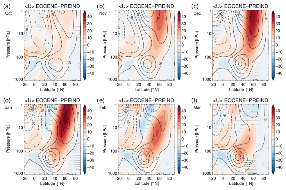
Figure 6Monthly evolution (October to March) of the zonal-mean zonal wind differences (m s−1) between the Eocene and preindustrial conditions in the Northern Hemisphere. Dotted regions indicate that anomalies are insignificantly different at the 5 % confidence level according to a t test. Black isolines shows the climatology derived from the preindustrial experiment.
At first glance, the strengthening of the polar vortex under Eocene conditions may seem inconsistent with the global acceleration of the Brewer–Dobson circulation as diagnosed by the younger stratospheric age of air (Fig. 2c). Indeed, a faster Brewer–Dobson circulation is associated with a stronger planetary wave drag in the stratosphere (i.e., an enhanced wave breaking), which in turn should lead to a weaker polar vortex. In the following, we hence investigate the seasonality of the planetary stationary wave activity and its interaction with the mean flow by calculating the Eliassen–Palm flux (hereafter EP flux) divergence, here scaled to units of zonal acceleration (Andrews et al., 1987):
where F is the EP flux whose components are
f is the Coriolis parameter, a is the Earth's radius, θ is the potential temperature, ρ0 is the density profile of the atmosphere and are the three-dimensional velocity components in spherical coordinates , where z is the log pressure. Overbars indicate zonal mean and primes denote departure from the zonal mean. As shown by Edmon et al. (1980), the EP flux constitutes a measure of the Rossby wave propagation from one height (z) and latitude (ϕ) to another, and its divergence (divEP) gives information about the forcing of the mean flow by the eddies.
Figure 7 displays the monthly evolution in winter of the EP flux and its divergence for the preindustrial conditions experiment. This analysis shows that, throughout winter, the wave activity penetrates the stratosphere (as indicated by the vectors) near 55∘ N, propagates upward and tends to be increasingly refracted toward the Equator with height. The dissipation of planetary waves exerts a westward-momentum forcing on the mean flow between 30 and 70∘ N (as diagnosed by the Eliassen–Palm flux convergence), which maximizes along the equatorward flank of the polar night jet where planetary wave breaking is large. This contributes to eroding and weakening the polar vortex and to a warming of the polar stratosphere and drives a persistent poleward mass transport in order to conserve the angular momentum. By mass continuity, this induces an upward transport at low latitudes and an extratropical downwelling (hence driving the Brewer–Dobson circulation). Under preindustrial climate conditions, we note that the wave activity and its interaction with the mean flow peaks in December or January (Fig. 7c, d) but is already large in November (Fig. 7b). Therefore, this contributes to slow down the radiatively driven development of the polar vortex in early winter.
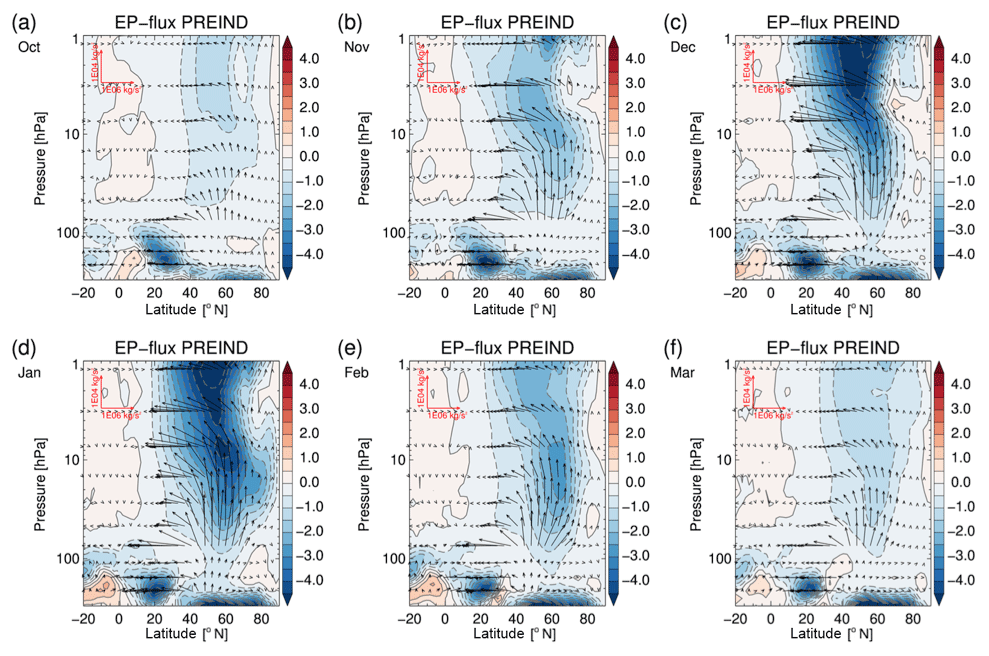
Figure 7Monthly evolution (October to March) of the Eliassen–Palm flux (vectors) and its divergence (contours, in m s −1 d−1) under preindustrial conditions in the Northern Hemisphere.
As shown in Fig. 8, under Eocene conditions, it appears that the planetary wave activity penetrating the stratosphere in early winter (i.e., November–December; Fig. 8b, c) is significantly reduced and deflected equatorward as revealed by the downward and equatorward pointing of the EP flux vector in the lower midlatitude stratosphere. This is associated with an anomalous positive EP flux divergence (i.e., a reduced convergence) throughout the depth of the stratospheric polar night jet (near 60∘ N), which indicates a substantially reduced westward-momentum forcing by planetary waves and hence allows a stronger development of the polar vortex in early winter in comparison with preindustrial conditions. In contrast, from January (Fig. 8d), the planetary wave activity becomes significantly larger under Eocene conditions, the westward forcing appears to be strongly amplified in the upper stratosphere and to progressively propagate downward in February (Fig. 8e). This is consistent with the reversal of the zonal-mean zonal wind anomaly in the upper stratosphere, but also with the overall extremely rapid deceleration of the polar-vortex strength noted previously (see Figs. 6 and S2). In addition, we analyzed the residual mass circulation (not shown) derived from the transformed Eulerian-mean formalism (Andrews et al., 1987). While no clear changes in the strength of the Brewer–Dobson circulation are found in early winter between Eocene and preindustrial conditions, late winter (February–March) reveals an important acceleration in Eocene conditions, which is consistent with the much stronger wave forcing found throughout the extratropical stratosphere (Fig. 8e, f). These results are consistent with a net acceleration of the Brewer–Dobson under Eocene conditions in comparison with preindustrial conditions as revealed by the younger age of air (Fig. 2c). Note that the Brewer–Dobson acceleration appears to be more pronounced in the Northern Hemisphere, where the mean flow and wave activity anomalies are found to be stronger than in the Southern Hemisphere (not shown).
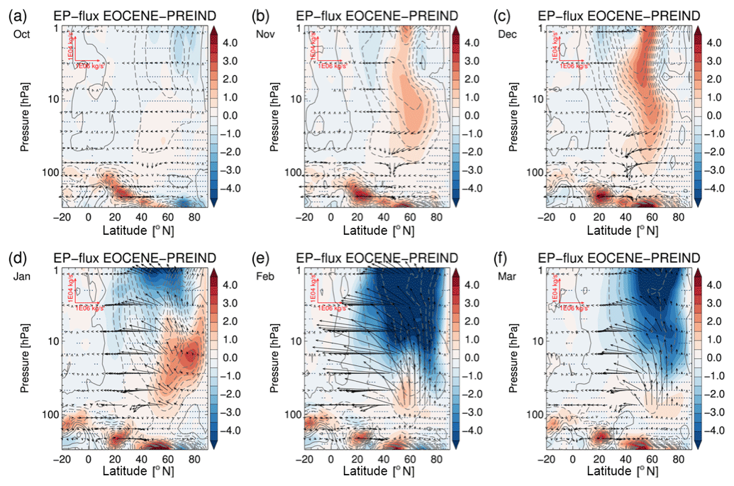
Figure 8Monthly evolution (October to March) of the differences between the Eocene and preindustrial conditions of the Eliassen–Palm flux and its divergence. Dotted regions indicate that anomalies are insignificantly different at the 5 % confidence level according to a t test. Preindustrial climatology is shown with dashed contours.
Although the large changes in the background state stratospheric circulation and its seasonal evolution under Eocene conditions in comparison with preindustrial climate conditions appear to be largely wave-driven, the origin of the identified changes in the planetary wave activity and its interaction with the mean flow remains to be determined. Note that this does not uniquely depend on changes in tropospheric wave sources but also on changes in the background flow itself, which modulates the wave propagation and the nature of wave-mean flow interactions. The planetary wave activity entering the stratosphere can be altered by numerous factors such as sea surface temperature changes (e.g., Hu et al., 2014), sea-ice changes (e.g., Kim et al., 2014), wind changes near the tropopause (e.g., Shepherd and McLandress, 2011; Karpechko and Manzini, 2017) or topography (Shi et al., 2014). Additional simulations of the Eocene and the preindustrial period with the atmospheric model (LMDz) without interactive chemistry and with a flat topography reveal that changes in the topography have first-order effects on planetary wave activity and hence on the stratospheric dynamics (not shown). Between the Eocene and the preindustrial conditions, beside large changes in the topography, important changes in air–sea thermal contrasts, sea-ice cover and sea surface temperature could all have a substantial influence on stratospheric circulation. The complexness of these effects and their possible interactions make an unambiguous attribution impossible in the absence of a dedicated experimental protocol that is out of the scope for the present study.
Model results shown in the previous section suggest that stratospheric dynamics and composition were very significantly altered under Eocene hot conditions in comparison with preindustrial climate conditions. In turn, these stratospheric changes may also have influenced the establishment of Eocene climate. Nowack et al. (2015) have shown that stratospheric changes driven by ozone changes can have an impact on the climate sensitivity in the context of high GHG concentrations for present-day conditions. The importance of this stratospheric ozone–climate feedback has, however, not been assessed in the context of Eocene hot climate. In this section, we estimate the role of this feedback on the overall Eocene climate response by comparing the EOCENE experiment (i.e., where ozone is calculated interactively and, hence, is physically consistent with Eocene conditions) with Eocene_OzRoyer and Eocene_Oz1855 experiments (i.e., where preindustrial ozone climatologies are prescribed in Eocene simulations). The latter simulations follow the protocol usually recommended for simulating paleoclimates (e.g., Kageyama et al., 2017).
Table 2 shows the total ozone and temperature changes as well as the effective radiative forcings induced by the use of an interactive stratospheric chemistry instead of seasonally varying prescribed climatologies. All the results in this section are discussed in terms of 25-year means. The effective radiative forcing is computed as the difference of net radiative flux at the top of atmosphere (TOA) between two atmospheric simulations (with ozone calculated interactively – with ozone climatology) as defined in Fig. 8.1.d of Myhre et al. (2013).
Table 2Global change in total column ozone, temperature and effective radiative forcings induced by the use of an interactive stratospheric chemistry instead of climatologies.
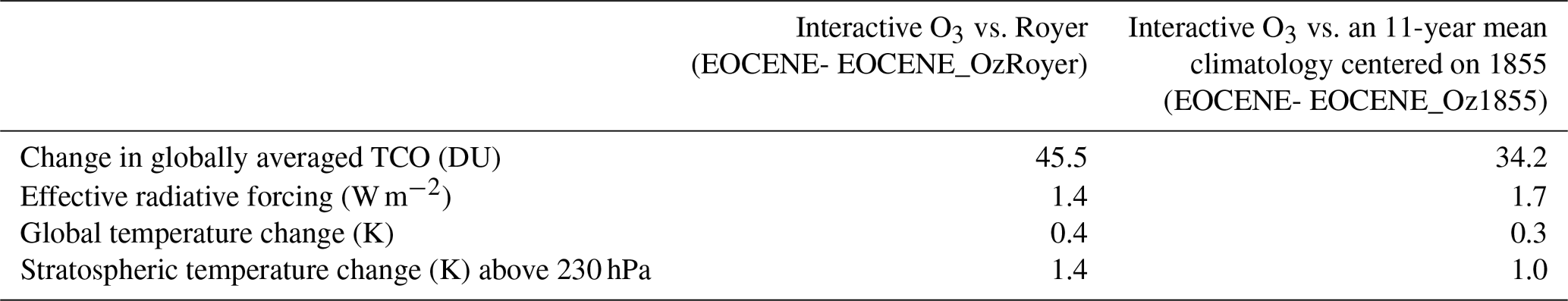
Figure 9 shows the distribution of total column ozone as a function of latitude for the different configurations. The preindustrial ozone distribution computed by REPROBUS and the Szopa et al. (2013) ozone climatology are represented as well. Comparing only the different preindustrial ozone distributions, the TCO in the experiment with the interactive calculation of ozone (PREIND in black) is higher than those of the climatologies (OzRoyer in blue, Oz1855 in brown). In addition, the interactive calculation of Eocene ozone (EOCENE in red) leads to much higher TCO than in the preindustrial climatologies (blue, brown), the 2000 climatology (green) and the preindustrial interactive ozone simulation (black). The global mean TCO is increased by about 45 or 35 DU with respect to the preindustrial OzRoyer or Oz1855 climatologies, respectively. For the sake of comparison, the global mean TCO had decreased by about 13 DU only between the 1960s and the end of the 1990s because of the past emissions of anthropogenic halogenated compounds, and the expected TCO increase at the 2100 horizon is projected to be between 13 and 32 DU depending on future anthropogenic emissions of GHGs (Bekki et al., 2013; Szopa et al., 2013). Taking the ozone distribution calculated in the EOCENE simulation as the reference, the TCO bias in an inappropriate ozone climatology can be 2 times higher (in the case of the OzRoyer climatology) than the TCO change calculated by the model between Eocene and preindustrial conditions (EOCENE versus PREIND; see Sect. 3).
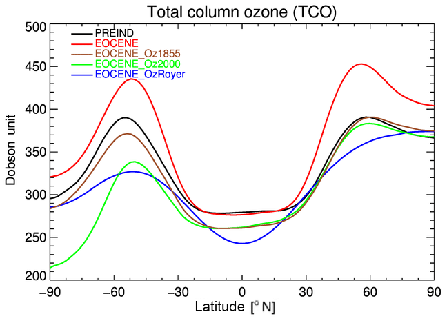
Figure 9Latitudinal distribution of ozone considered by the circulation model LMDz when using climatologies from Royer (blue), from Szopa et al. (2013) centered on the year 2000 (green) or centered on the year 1855 (maroon) or interactively computed by REPROBUS for Eocene conditions (red) or preindustrial conditions (black).
The TCO difference between the EOCENE ozone distribution and ozone climatologies peak at midlatitudes (about 40∘), reaching almost 70 DU for the Oz1855 climatology and about 100 DU for the OzRoyer climatology (Fig. 10a). In order to identify the regions responsible for the general increase in TCO calculated from preindustrial to Eocene conditions, the zonal mean distributions of ozone difference between EOCENE and Oz1855 climatologies are plotted in DU km−1 in Fig. 10b. The TCO increase in EOCENE is largely due to an enhancement in ozone in the upper stratosphere. The TCO change in the tropics is very moderate because the upper-stratospheric ozone enhancements are more or less compensated for by lower-stratospheric ozone decreases brought about by the acceleration of the Brewer–Dobson circulation, namely the faster ascent in the tropics (Sect. 3). TCO enhancements peak at midlatitudes because the ozone concentration increases reach down to 150 hPa at midlatitudes, again certainly linked to the acceleration of the Brewer–Dobson circulation and more specifically the faster descent at mid- and high latitudes. Below 200 hPa, around the tropopause region, extratropical EOCENE ozone concentrations are lower than in the Oz1855 climatology, mostly because of the rise in the tropopause height (Sect. 3).
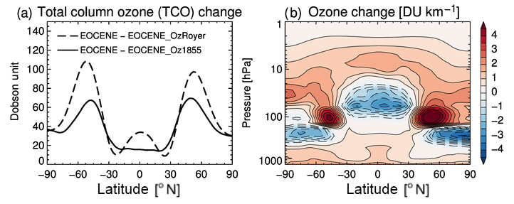
Figure 10Total column ozone (TCO) changes (in Dobson units or DU) between the EOCENE simulation and the EOCENE-Oz1855 simulation (considering the 1855 ozone climatology) (a) and TCO changes between the EOCENE simulation and the two climate-only simulations considering the (solid) 1855 ozone climatology and (dashed) Royer ozone parameterization (b).
Ozone changes naturally lead to temperature changes, especially in the stratosphere where ozone and temperature are closely coupled. Figure 11 shows the zonal mean distribution of temperature difference between EOCENE and EOCENE_Oz1855 simulations. The impact is weak below 400 hPa since SSTs are fixed and identical in all the Eocene simulations (EOCENE, EOCENE_OzRoyer, EOCENE_Oz1855). The change in zonal mean temperatures below 400 hPa does not exceed 0.15 K but can almost reach 0.5 K for the northern polar latitudes when the interactive ozone simulation (EOCENE) is compared to the EOCENE_OzRoyer (not shown). In contrast, temperatures above about 200 hPa are significantly impacted by the choice of ozone distribution used in the model. Temperatures are more than 2.5 to 3 K higher at middle and high latitudes in both hemispheres when ozone is calculated interactively instead of using the preindustrial 1855 climatology. The largest differences are found near the stratopause region (above 5 hPa), in the lower polar lower stratosphere(∼130 hPa) and in the middle tropical stratosphere (∼60 hPa), where temperatures are, respectively, higher than 6 K, higher than 4 K and lower than 3.5 K in the simulation with interactive ozone compared to the one with the preindustrial climatology.
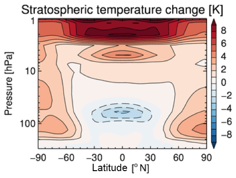
Figure 11Stratospheric temperature changes (K) between the EOCENE simulation and the climate-only simulation with the 1855 ozone climatology.
5.1 Impact on climate
The consideration of a stratospheric ozone compatible with the Eocene conditions perturbs the radiative balance compared to the use of a preindustrial climatology. The net radiative change (shortwave + longwave) between the simulation with interactive chemistry and the simulation with preindustrial climatology corresponds to a 1.7 W m−2 effective radiative forcing (RF). This radiative forcing results from combined positive RFs in the longwave (LW) and shortwave (SW) simulated in the tropics. Beyond 50∘ (north and south), the positive SW RF is partly counterbalanced by a negative longwave RF (see Table 3 and Fig. 12). This radiative forcing from the stratospheric ozone response represents a positive climate feedback, which is commonly ignored in Eocene climate simulations. In order to estimate the potential impact of an interactive ozone on surface temperature under Eocene conditions, we consider a large range of climate sensitivity from 0.4 to 1.2 K (W m−2)−1 (Knutti et al., 2017). Given such a broad range, the surface temperature response to this stratospheric forcing could range from 0.7 to 2.0 K (assuming an effective radiative forcing of 1.7 W m−2). The surface temperature response to a specific radiative forcing depends on the considered climate conditions and on the nature of the climate forcer. Considering an interactive stratospheric ozone chemistry under a 4×CO2 climate perturbation, Nowack et al. (2015) found a climate sensitivity of 1.05 K (W m−2)−1 in their ESM. Applying this climate sensitivity, the surface temperature change associated with the ozone feedback would be about 1.8 K when considering interactive stratospheric chemistry (compared with the EOCENE_Oz1855 run). The climate sensitivity to ozone change can obviously vary from one ESM to another since, for example, the sensitivity of the Brewer–Dobson circulation to climate is highly model-dependant (SPARC CCMVal, 2010). Nonetheless, this estimation allows us to discuss the importance of considering this chemistry–climate feedback when attempting to simulate greenhouse paleoclimates. According to the IPCC AR5 report (IPCC, 2013), the global land surface air temperature anomaly is +12.7 K for the early Eocene climatic optimum (Masson-Delmotte et al., 2013). This estimation is based on simulations from several models analyzed by Lunt et al. (2012), for which there was no common modeling protocol (e.g., CO2 being in the 2×[CO2]PI to 16×[CO2]PI range). One of these models, the HadCM model, estimates that the effect of changing non-CO2 boundary conditions (topography, bathymetry, solar constant and vegetation) for Eocene conditions leads to a 1.8 K increase in the global mean surface air temperature (to be compared to a 3.3 K increase when doubling the CO2). The feedback of stratospheric ozone on surface air temperature could thus represent about 15 % of the total temperature anomaly reported between Eocene and preindustrial conditions and be as important as the effect of external forcings.
Table 3Differences in shortwave and longwave radiative fluxes at different vertical levels between the EOCENE simulation and the climate-only simulation with the 1855 ozone climatology.
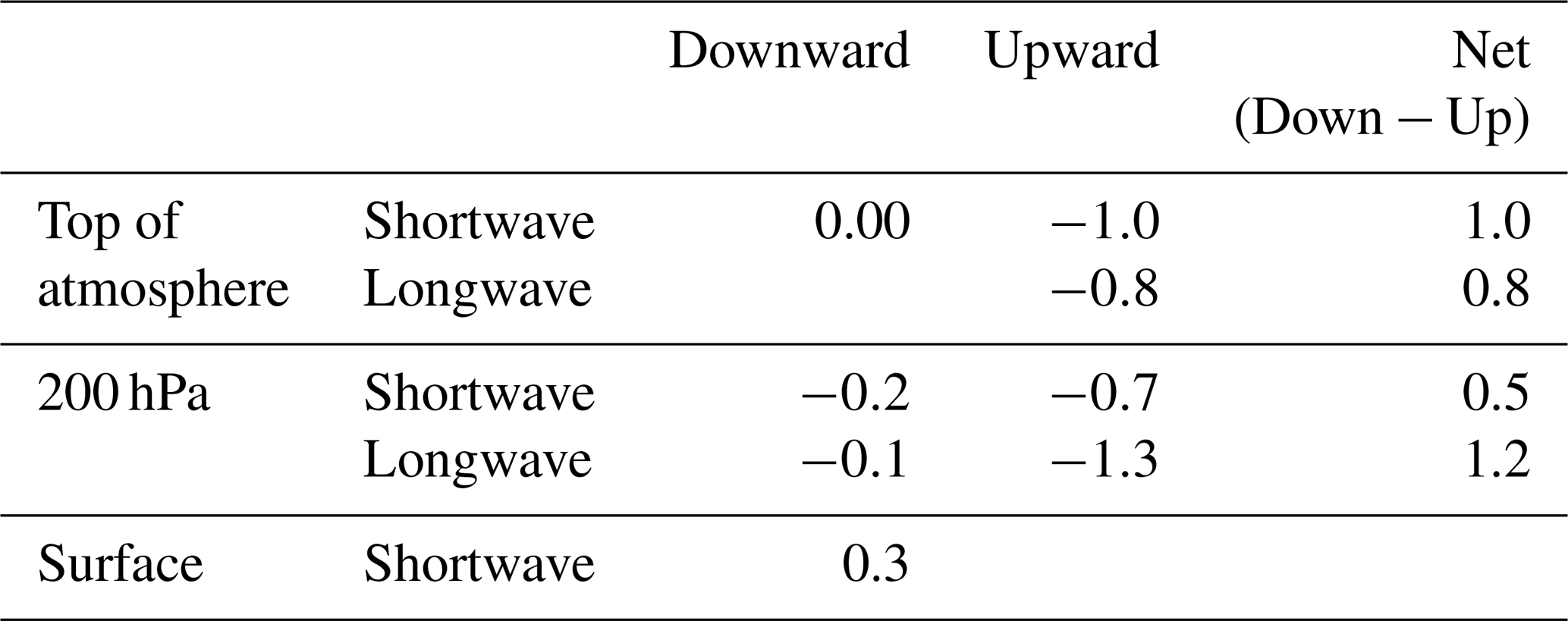
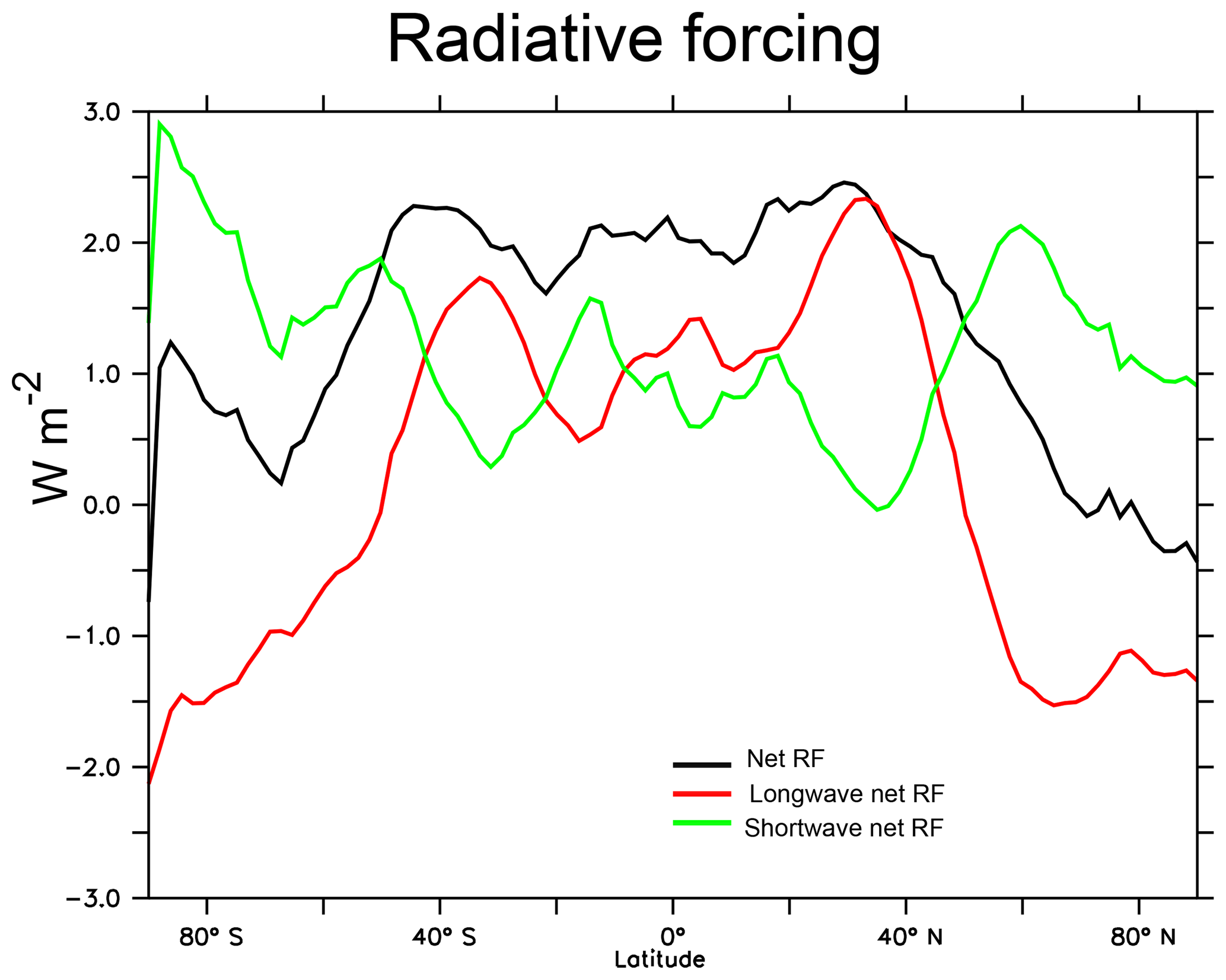
Figure 12Differences in radiative fluxes as a function of latitude between the EOCENE simulation and the climate-only simulation with the 1855 ozone climatology.
In strong greenhouse climate, the terrestrial carbon and nitrogen cycles are intensified, releasing high CH4 and N2O in the atmosphere (Beerling et al., 2011). The effect of changing N2O and CH4 in the troposphere (including the H2O increase in the stratosphere induced by the CH4 increase) has been assessed by Beerling et al. (2011). These authors find, with the STOCHEM model, a 2.1 K increase in global surface temperature due solely to the tropospheric composition changes. Our results suggest that the effect of the stratospheric ozone feedback on surface temperatures is of similar importance.
5.2 Impact on tropospheric conditions
Using an ESM including chemistry, Unger and Yue (2014) found that under warm and high methane Pliocene conditions, the stratospheric ozone burden was 5 % higher than the preindustrial one. This stratospheric ozone increase resulted in a 20 % reduction in the tropospheric photolysis rate of ozone () that leads to the formation of OH, the hydroxyl radical. This radical is the main oxidant of the troposphere and its decrease (of 20 % to 25 % in the Unger and Yue simulations) impacts the lifetime of chemical species and in particular CH4. Our simulations show a 7.2 % increase in the stratospheric ozone burden when comparing the EOCENE and the PREIND simulation (both including interactive chemistry) and an 8.8 % difference when comparing the EOCENE simulation to the EOCENE_Oz1855.
In addition, we estimate the change in surface UV radiations and ozone photolysis in the Eocene conditions. Using the radiation transfer model Quick TUV Calculator with a pseudo-spherical discrete ordinate four streams (http://cprm.acom.ucar.edu/Models/TUV/Interactive_TUV/, last access: 2 June 2019), we estimate the effect of the stratospheric ozone increase on the ozone photolysis, which controls the OH production. Considering a 65 DU change at a 50∘ latitude (corresponding to the maximum of Fig. 10), the photolysis rate at the surface decreases by 25 %. A decrease in the ozone photolysis rate would induce a significant decrease in OH and hence in the tropospheric oxidizing capacity, thus making CH4 longer lived and reinforcing its effect on climate. It would also impact the overall tropospheric chemistry.
The stratospheric dynamics and ozone layer respond to – and interact with – atmospheric variations (climate, tropospheric GHG content). In this study, we simulate these interactions in the case of the hot Eocene climate using a chemistry–climate model. We characterize the changes in ozone and middle-atmospheric dynamics-induced hot Eocene climate conditions characterized by a 4×CO2 climate, elevated concentrations of CH4 and N2O, and substantial changes in surface boundary conditions (e.g., sea surface temperature, sea-ice cover or topography) compared to preindustrial climate. The climate impact of the stratospheric response under hot conditions is also discussed.
Comparing the Eocene simulation with a preindustrial simulation, we find a sharp increase in ozone in the upper stratosphere (reaching 40 % at 2–3 hPa in the tropics) linked to the strong cooling of the stratosphere (up to −12 K at 10 hPa), which slows down the chemical destruction of ozone. Meanwhile, ozone is greatly reduced in the lower tropical stratosphere (up to 40 %) due to the intensification of Brewer–Dobson circulation. These results are in agreement with previous modeling studies that considered current tropospheric composition and a 4×CO2 climate change.
As a consequence of the opposite ozone changes in the tropics (enhanced ozone in the upper stratosphere, reduced ozone in the lower stratosphere), the tropical total column ozone (TCO) is not affected much by the difference in climate between the Eocene and preindustrial periods. On the contrary, at midlatitudes and, to a lesser extent, in the polar regions, the TCO is considerably increased. The TCO meridional distribution is also strongly modified, exhibiting particularly pronounced midlatitude maxima and a steeper negative poleward gradient from these maxima. These changes in meridional distribution reflect significant polar-vortex changes during the winter or early spring, especially in the Northern Hemisphere. The polar vortex becomes stronger and more extended equatorward under Eocene conditions, thus reinforcing the isolation of the polar-vortex air masses from the midlatitudes in comparison with preindustrial conditions. In our simulations, the reinforcement of the stratospheric polar vortex under Eocene conditions and the acceleration of the stratospheric overturning circulation (which seems contradictory at first) is consistent with a reduced intensity of the planetary wave activity and its interaction with the mean flow in early winter and, conversely, a strongly amplified wave activity and interaction with the mean flow in late winter compared to preindustrial conditions.
We then explore the possible role of the stratospheric ozone response in the establishment of Eocene climate. For that purpose, we compare the simulations with interactive ozone with simulations forced by the use of preindustrial ozone climatologies. The difference in global mean TCO between the Eocene simulation and simulations using preindustrial climatologies is 2 to 3 times higher than the change in ozone observed between 1960 and end of the 1990s (the minimum TCO) and of the same order as the changes projected between 2000 and 2100. The ozone increase in the upper stratosphere in the case of Eocene interactive ozone warms the atmosphere by up to 3 K above 230 hPa. In the tropical lower stratosphere, zonal mean temperatures are up to 3.5 K lower for the Eocene stratospheric ozone compared to the preindustrial ozone. These changes in the thermal structure of the middle atmosphere could, via atmospheric circulation teleconnections, have significant regional consequences. Using the sensitivity of surface temperatures to stratospheric ozone changes determined by Nowack et al. (2015) (though climate sensitivity varies among climate–chemistry models), we estimate the contribution of stratospheric ozone feedback to surface temperature change in Eocene hot climate simulations. We find that it is potentially as important as the effects of non-CO2 boundary conditions (topography, bathymetry, solar constant and vegetation) or uncertainties due to gaseous tropospheric chemistry. The results suggest that future studies exploring long-standing Cenozoic warm-climate questions, such as the varying latitudinal temperature gradient during hothouse periods, would benefit from exploring and integrating – even if costly in terms of computing time – the feedbacks of ozone on atmospheric temperatures rather than prescribing preindustrial values.
The main model outputs are publicly accessible at https://doi.org/10.14768/201906141.01 (Szopa et al., 2019).
The supplement related to this article is available online at: https://doi.org/10.5194/cp-15-1187-2019-supplement.
The idea of the study, the design of numerical simulations and the radiative forcing analysis come from SS. RT performed all the analysis on atmospheric dynamics. SvB provided the Eocene boundary conditions. SS and RT prepared the first draft of the paper. All coauthors contributed to its editing.
The authors declare that they have no conflict of interest.
The authors are thankful to the NCAR Atmospheric Chemistry Division (ACD) for the distribution of the NCAR/ACD TUV: Tropospheric Ultraviolet & Visible Radiation Model (http://cprm.acom.ucar.edu/Models/TUV/Interactive_TUV/) and the availability of their quicktool. We thank Yannick Donnadieu for preparing the paleogeographical conditions for Eocene simulations and Marion Marchand for her advice in the use of the REPROBUS model and Jean-Louis Dufresne for helpful discussion on radiative forcing.
This research has been supported by the Agence Nationale de la Recherche (PALEOx project, grant no. ANR-16-CE31-0010). This work was granted access to the HPC resources of TGCC under the allocation 2017-A0050102212 made 40 by GENCI (Grand Equipement National de Calcul Intensif).
This paper was edited by Arne Winguth and reviewed by two anonymous referees.
Anagnostou, E., John, E., Edgar, K., Foster, G., Ridgwell, A., Inglis, G., Pancost, R., Lunt, D., and Pearson, P.: Changing atmospheric CO2 concentration was the primary driver of early Cenozoic climate, Nature, 533, 380–384, https://doi.org/10.1038/nature17423, 2016.
Andrews, D. G., Holton, J. R., and Leovy, C. B.: Middle Atmospheric Dynamics, Academic Press, San Diego, 489 pp, 1987.
Avallone, L. M. and Prather, M. J.: Photochemical evolution of ozone in the lower tropical stratosphere, J. Geophys. Res.-Atmos., 101, 1457–1461, https://doi.org/10.1029/95JD03010, 1996.
Ayarzagüena, B., Polvani, L. M., Langematz, U., Akiyoshi, H., Bekki, S., Butchart, N., Dameris, M., Deushi, M., Hardiman, S. C., Jöckel, P., Klekociuk, A., Marchand, M., Michou, M., Morgenstern, O., O'Connor, F. M., Oman, L. D., Plummer, D. A., Revell, L., Rozanov, E., Saint-Martin, D., Scinocca, J., Stenke, A., Stone, K., Yamashita, Y., Yoshida, K., and Zeng, G.: No robust evidence of future changes in major stratospheric sudden warmings: a multi-model assessment from CCMI, Atmos. Chem. Phys., 18, 11277–11287, https://doi.org/10.5194/acp-18-11277-2018, 2018.
Baatsen, M., von der Heydt, A. S., Huber, M., Kliphuis, M. A., Bijl, P. K., Sluijs, A., and Dijkstra, H. A.: Equilibrium state and sensitivity of the simulated middle-to-late Eocene climate, Clim. Past Discuss., https://doi.org/10.5194/cp-2018-43, in review, 2018.
Beerling, D. J., Fox, A., Stevenson, D. S., and Valdes, P. J.: Enhanced chemistry-climate feedbacks in past greenhouse worlds, P. Natl. Acad. Sci. USA, 108, 9770–9775, https://doi.org/10.1073/pnas.1102409108, 2011.
Bekki, S., Bodeker, G. E., Bais, A. F., Butchart, N., Eyring, V., Fahey, D. W., Kinnison, D. E., Langematz, U., Mayer, B., Portmann, R. W., Rozanov, E., Braesicke, P., Charlton-Perez, A. J., Chubarova, N. E., Cionni, I., Diaz, S. B., Gillett, N. P., Giorgetta, M. A., Komala, N., Lefèvre, F., McLandress, C., Perlwitz, J., Peter, T., and Shibata, K.: Future Ozone and Its Impact on Surface UV, Chapter 3 in: Scientific Assessment of Ozone Depletion: 2010, Global Ozone Research and Monitoring Project–Report No. 52, 516 pp., World Meteorological Organization, Geneva, Switzerland, 2011.
Bekki, S., Rap, A., Poulain, V., Dhomse, S., Marchand, M., Lefèvre, F., Forster, P. M., Szopa, S., and Chipperfield, M. P.: Climate impact of stratospheric ozone recovery. Geophys. Res. Lett., 40, 2796–2800, 2013.
Botsyun, S., Sepulchre, P., Donnadieu, Y., Risi, C., Licht, A., and Caves Rugenstein, J. K. : Revised paleoaltimetry data show low Tibetan plateau elevation during the Eocene, Science, 363, eaaq1436, https://doi.org/10.1126/science.aaq1436, 2019.
Brasseur, G. P. and Solomon, S.: Aeronomy of the Middle Atmosphere: Chemistry and Physics of the Stratosphere and Mesosphere, 644 pp., 3rd rev. and enlarged ed., Springer, the Netherlands, 2005.
Butchart, N.: The Brewer–Dobson circulation, Rev. Geophys., 52, 157–184, https://doi.org/10.1002/2013RG000448, 2014.
Chiodo, G. and Polvani, L. M.: Reduced Southern Hemispheric circulation response to quadrupled CO2 due to stratospheric ozone feedback, Geophys. Res. Lett., 44, 465–474, https://doi.org/10.1002/2016GL071011, 2017.
Chiodo, G., Polvani, L. M., Marsh, D. R., Stenke, A., Ball, W., Rozanov, E., Muthers, S., and Tsigaridis, K.: The response of the ozone layer to quadrupled CO2 concentrations, J. Climate, https://doi.org/10.1175/JCLI-D-17-0492.1, 2018.
Chipperfield, M. P., Bekki, S., Dhomse, S., Harris, N. R. P., Hassler, B., Hossaini, R., Steinbrecht, W., Thiéblemont, R., and Weber, M.: Detecting recovery of the stratospheric ozone layer, Nature, 549, 211–218, 2017.
de la Cámara, A., Lott, F., and Abalos, M.: Climatology of the middle atmosphere in LMDz: Impact of source-related parameterizations of gravity wave drag, J. Adv. Model. Earth Sy., 8, 1507– 1525, https://doi.org/10.1002/2016MS000753, 2016a.
de la Cámara, A., Lott, F., Jewtoukoff, V., Plougonven, R., and Hertzog, A.: On the gravity wave forcing during the southern stratospheric final warming in LMDz, J. Atmos. Sci., 73, 3213–3226, https://doi.org/10.1175/JAS-D-15-0377.1, 2016b.
Dietmüller, S., Ponater, M., and Sausen, R.: Interactive ozone induces a negative feedback in CO2-driven climate change simulations, J. Geophys. Res.-Atmos., 119, 1796–1805, https://doi.org/10.1002/2013JD020575, 2014.
Dufresne, J.-L., Foujols, M.-A., Denvil, S. , Caubel, A., Marti, O., Aumont, O., Balkanski, Y., Bekki, S., Bellenger, H., Benshila, R., Bony, S., Bopp, L., Braconnot, P., Brockmann, P., Cadule, P., Cheruy, F., Codron, F., Cozic, A., Cugnet, D., de Noblet, N., Duvel, J.-P., Ethé, C., Fairhead, L., Fichefet, T., Flavoni, S., Friedlingstein, P., Grandpeix, J.-Y., Guez, L., Guilyardi, E., Hauglustaine, D., Hourdin, F., Idelkadi, A., Ghattas, J., Joussaume, S., Kageyama, M., Krinner, G., Labetoulle, S., Lahellec, A., Lefebvre, M.-P., Lefevre, F., Levy, C., Li, Z. X., Lloyd, J., Lott, F., Madec, G., Mancip, M., Marchand, M., Masson, S., Meurdesoif, Y., Mignot, J., Musat, I., Parouty, S., Polcher, J., Rio, C., Schulz, M., Swingedouw, D., Szopa, S., Talandier, C., Terray, P., Viovy, N., and Vuichard, N.: Climate change projections using the IPSL-CM5 Earth System Model: from CMIP3 to CMIP5, Clim. Dynam., 40, 2123–2165, https://doi.org/10.1007/s00382-012-1636-1, 2013.
Edmon, H. J., Hoskins, B. J., and McIntyre, M. E.: Eliassen–Palm cross sections for the troposphere, J. Atmos. Sci., 37, 2600–2616, 1980.
Haigh, J. D. and Pyle, J. A.: Ozone perturbation experiments in a two-dimensional circulation model, Q. J. Roy. Meteorol. Soc., 109, 551–574, https://doi.org/10.1002/qj.49710845705, 1982.
Herold, N., Buzan, J., Seton, M., Goldner, A., Green, J. A. M., Müller, R. D., Markwick, P., and Huber, M.: A suite of early Eocene (∼55 Ma) climate model boundary conditions, Geosci. Model Dev., 7, 2077–2090, https://doi.org/10.5194/gmd-7-2077-2014, 2014.
Hourdin, F., Grandpeix, J. Y., Rio, C., Bony, S., Jam, A., Cheruy, F., Rochetin, N., Fairhead, L., Idelkadi, A., Musat, I., Dufresne, J.-L., Lefebvre, M.-P., Lahellec, A., and Roehrig, R.: LMDZ5B: the atmospheric component of the IPSL climate model with revisited parameterizations for clouds and convection, Clim. Dynam., 40, 2193, https://doi.org/10.1007/s00382-012-1343-y, 2013.
Hu, D. Z., Tian, W. S., Xie, F., Shu, J. C., and Dhomse, S.: Effects of meridional sea surface temperature changes on stratospheric temperature and circulation, Adv. Atmos. Sci., 31, 888–900, https://doi.org/10.1007/s00376-013-3152-6, 2014.
IPCC: Climate Change 2013: The Physical Science Basis. Contribution of Working Group I to the Fifth Assessment Report of the Intergovernmental Panel on Climate Change, edited by: Stocker, T. F., Qin, D., Plattner, G.-K., Tignor, M., Allen, S. K., Boschung, J., Nauels, A., Xia, Y., Bex, V., and Midgley, P. M., Cambridge University Press, Cambridge, UK and New York, NY, USA, 1535 pp., https://doi.org/10.1017/CBO9781107415324, 2013.
Jacob, R.: Low Frequency Variability in a Simulated Atmosphere Ocean System, PhD thesis, University of Wisconsin-Madison, Madison, WI, USA, 1997.
Jourdain, L., Bekki, S., Lott, F., and Lefèvre, F.: The coupled chemistry-climate model LMDz-REPROBUS: description and evaluation of a transient simulation of the period 1980–1999, Ann. Geophys., 26, 1391–1413, https://doi.org/10.5194/angeo-26-1391-2008, 2008.
Kageyama, M., Albani, S., Braconnot, P., Harrison, S. P., Hopcroft, P. O., Ivanovic, R. F., Lambert, F., Marti, O., Peltier, W. R., Peterschmitt, J.-Y., Roche, D. M., Tarasov, L., Zhang, X., Brady, E. C., Haywood, A. M., LeGrande, A. N., Lunt, D. J., Mahowald, N. M., Mikolajewicz, U., Nisancioglu, K. H., Otto-Bliesner, B. L., Renssen, H., Tomas, R. A., Zhang, Q., Abe-Ouchi, A., Bartlein, P. J., Cao, J., Li, Q., Lohmann, G., Ohgaito, R., Shi, X., Volodin, E., Yoshida, K., Zhang, X., and Zheng, W.: The PMIP4 contribution to CMIP6 – Part 4: Scientific objectives and experimental design of the PMIP4-CMIP6 Last Glacial Maximum experiments and PMIP4 sensitivity experiments, Geosci. Model Dev., 10, 4035–4055, https://doi.org/10.5194/gmd-10-4035-2017, 2017.
Karpechko, A. Y. and Manzini, E.: Arctic stratosphere dynamical response to global warming, J. Climate, 30, 7071–7086, https://doi.org/10.1175/JCLI-D-16-0781.1, 2017.
Keating, G. M. and Young, D. F.: Interim reference models for the middle atmosphere, Handbook for MAP, 16, 205–229, 1985.
Kim, B. M., Son, S. W., Min, S. K., Jeong, J. H., Kim, S. J., Zhang, X., Shim, T., and Yoon, J. H.: Weakening of the stratospheric polar vortex by Arctic sea-ice loss, Nat. Commun., 5, 4646, https://doi.org/10.1038/ncomms5646, 2014.
Knutti, R., Rugenstein, M. A. A., and Hegerl, G. C.: Beyond equilibrium climate sensitivity, Nat. Geosci., 10, 727–736, https://doi.org/10.1038/ngeo3017, 2017.
Krueger, A. J. and Minzner, R. A.: A Mid-Latitude Ozone Model for the 1976 U.S. Standard Atmosphere, J. Geophys. Res., 81, 4477–4481, 1976.
Ladant, J. B., Donnadieu, Y., Lefebvre, V., and Dumas, C.: The respective role of atmospheric carbon dioxide and orbital parameters on ice sheet evolution at the Eocene-Oligocene transition, Paleoceanography, 29, 810–823, https://doi.org/10.1002/2013PA002593, 2014.
Ladant, J.-B. and Donnadieu, Y.: Palaeogeographic regulation of glacial events during the Cretaceous supergreenhouse. Nat. Commun. 7, 12771, https://doi.org/10.1038/ncomms12771, 2016.
Lefèvre, F., Brasseur, G. P., Folkins, I., Smith, A. K., and Simon, P.: Chemistry of the 1991–1992 stratospheric winter: Three-dimensional model simulations, J. Geophys. Res., 199, 8183–8195, 1994.
Lefèvre, F., Figarol, F., Carslaw, K. S., and Peter, T.: The 1997 Arctic ozone depletion quantified from three-dimensional model simulations, Geophys. Res. Lett., 25, 2425–2428, 1998.
Li, F., Stolarski, R. S., and Newman, P. A.: Stratospheric ozone in the post-CFC era, Atmos. Chem. Phys., 9, 2207–2213, https://doi.org/10.5194/acp-9-2207-2009, 2009.
Licht, A., van Cappelle, M., Abels, H. A., Ladant, J.-B., Trabucho-Alexandre, J., France-Lanord, C., Donnadieu, Y., Vandenberghe, J., Rigaudier, T., Lécuyer, C., Terry Jr., D., Adriaens, R., Boura, A., Guo, Z., Aung Naing Soe, Quade, J., Dupont-Nivet, G., and Jaeger, J.-J.: Asian monsoons in a late Eocene greenhouse world, Nature, 513, 501–506, 2014.
Lunt, D. J., Dunkley Jones, T., Heinemann, M., Huber, M., LeGrande, A., Winguth, A., Loptson, C., Marotzke, J., Roberts, C. D., Tindall, J., Valdes, P., and Winguth, C.: A model–data comparison for a multi-model ensemble of early Eocene atmosphere–ocean simulations: EoMIP, Clim. Past, 8, 1717–1736, https://doi.org/10.5194/cp-8-1717-2012, 2012.
Lunt, D. J., Huber, M., Anagnostou, E., Baatsen, M. L. J., Caballero, R., DeConto, R., Dijkstra, H. A., Donnadieu, Y., Evans, D., Feng, R., Foster, G. L., Gasson, E., von der Heydt, A. S., Hollis, C. J., Inglis, G. N., Jones, S. M., Kiehl, J., Kirtland Turner, S., Korty, R. L., Kozdon, R., Krishnan, S., Ladant, J.-B., Langebroek, P., Lear, C. H., LeGrande, A. N., Littler, K., Markwick, P., Otto-Bliesner, B., Pearson, P., Poulsen, C. J., Salzmann, U., Shields, C., Snell, K., Stärz, M., Super, J., Tabor, C., Tierney, J. E., Tourte, G. J. L., Tripati, A., Upchurch, G. R., Wade, B. S., Wing, S. L., Winguth, A. M. E., Wright, N. M., Zachos, J. C., and Zeebe, R. E.: The DeepMIP contribution to PMIP4: experimental design for model simulations of the EECO, PETM, and pre-PETM (version 1.0), Geosci. Model Dev., 10, 889–901, https://doi.org/10.5194/gmd-10-889-2017, 2017.
Masson-Delmotte, V., Schulz, M., Abe-Ouchi, A., Beer, J., Ganopolski, A., González Rouco, J. F., Jansen, E., Lambeck, K., Luterbacher, J., Naish, T. R., Osborn, T., Otto-Bliesner, B. L., Quinn, T. M., Ramesh, R., Rojas, M., Shao, X. M., and Timmermann, A.: Information from Paleoclimate, Archives, in: Climate Change 2013: The Physical Science Basis, Contribution of WG I to the Fifth Assessment Report of the IPCC, edited by: Stocker, T.F., Qin, D., Plattner, G.-K., Tignor, M., Allen, S. K., Boschung, J., Nauels, A., Xia, Y., Bex, V., and Midgley, P. M., Cambridge University Press, Cambridge, United Kingdom and New York, NY, USA, 383–464, http://www.ipcc.ch/report/ar5/wg1/#.UvIJHPl5MqI (last access: 14 June 2019), 2013.
McLandress, C., Shepherd, T. G., Scinocca, J. F., Plummer, D. A., Sigmond, M., Jonsson, A. I., and Reader, M. C.: Separating the Dynamical Effects of Climate Change and Ozone Depletion, Part II: Southern Hemisphere Troposphere, J. Climate, 24, 1850–1868, https://doi.org/10.1175/2010JCLI3958.1, 2011.
Morgenstern, O., Hegglin, M. I., Rozanov, E., O'Connor, F. M., Abraham, N. L., Akiyoshi, H., Archibald, A. T., Bekki, S., Butchart, N., Chipperfield, M. P., Deushi, M., Dhomse, S. S., Garcia, R. R., Hardiman, S. C., Horowitz, L. W., Jöckel, P., Josse, B., Kinnison, D., Lin, M., Mancini, E., Manyin, M. E., Marchand, M., Marécal, V., Michou, M., Oman, L. D., Pitari, G., Plummer, D. A., Revell, L. E., Saint-Martin, D., Schofield, R., Stenke, A., Stone, K., Sudo, K., Tanaka, T. Y., Tilmes, S., Yamashita, Y., Yoshida, K., and Zeng, G.: Review of the global models used within phase 1 of the Chemistry–Climate Model Initiative (CCMI), Geosci. Model Dev., 10, 639–671, https://doi.org/10.5194/gmd-10-639-2017, 2017.
Myhre, G., Shindell, D., Bréon, F.-M., Collins, W., Fuglestvedt, J., Huang, J., Koch, D., Lamarque, J.-F., Lee, D., Mendoza, B., Nakajima, T., Robock, A., Stephens, G., Takemura, T., and Zhang, H.: Anthropogenic and Natural Radiative Forcing. In: Climate Change 2013: The Physical Science Basis. Contribution of Working Group I to the Fifth Assessment Report of the Intergovernmental Panel on Climate Change, edited by: Stocker, T. F., Qin, D., Plattner, G.-K., Tignor, M., Allen, S. K., Boschung, J., Nauels, A., Xia, Y., Bex, V., and Midgley, P. M., Cambridge University Press, Cambridge, UK and New York, NY, USA, 2013.
Nowack, P. J., Abraham, N. L., Maycock, A. C., Braesicke, P., Gregory, J. M., Joshi, M. M., Osprey, A., and Pyle, J. A.: A large ozone-circulation feedback and its implications for global warming assessments, Nat. Clim. Change, 5, 41–45, https://doi.org/10.1038/NCLIMATE2451, 2015.
Pohl, A., Donnadieu, Y., Le Hir, G., Ladant, J.-B., Dumas, C., Alvarez-Solas, J., and Vandenbroucke, T. R. A.: Glacial onset predated Late Ordovician climate cooling, Paleoceanography, 31, 800–821, https://doi.org/10.1002/2016PA002928, 2016.
Porada, P. T., Lenton, M., Pohl, A., Weber, B., Mander, L., Donnadieu, Y., Beer, C., Pöschl, U., and Kleidon, A.: High potential for weathering and climate effects of non-vascular vegetation in the Late Ordovician, Nat. Commun., 7, 12113, https://doi.org/10.1038/ncomms12113, 2016.
Revell, L. E., Bodeker, G. E., Huck, P. E., Williamson, B. E., and Rozanov, E.: The sensitivity of stratospheric ozone changes through the 21st century to N2O and CH4, Atmos. Chem. Phys., 12, 11309–11317, https://doi.org/10.5194/acp-12-11309-2012, 2012.
Sassi, F., Boville, B. A., Kinnison, D., and Garcia, R. R.: The effects of interactive ozone chemistry on simulations of the middle atmosphere, Geophys. Res. Lett., 32, L07811, https://doi.org/10.1029/2004GL022131, 2005.
Sausen, R. and Santer, B. D.: Use of changes in tropopause height to detect influences on climate, Meteorol. Z., 12, 131–136, 2003.
Shepherd, T. G. and McLandress, C.: A robust mechanism for strengthening of the Brewer–Dobson circulation in response to climate change: critical-layer control of subtropical wave breaking, J. Atmos. Sci., 68, 784–797, https://doi.org/10.1175/2010JAS3608.1, 2011.
Shi, Z., Liu, X., Liu, Y., Sha, Y., and Xu, T.: Impact of Mongolian Plateau versus Tibetan Plateau on the westerly jet over North Pacific Ocean, Clim. Dynam., 44, 3067–3076, 2014.
Sitch, S., Smith, B., Prentice, I. C., Arneth, A., Bondeau, A., Cramer, W., Kaplan, J. O., Levis, S., Lucht, W., Sykes, M. T., Thonicke, K., and Venevsky, S.: Evaluation of ecosystem dynamics, plant geography and terrestrial carbon cycling in the LPJ dynamic vegetation model, Glob. Change Biol., 9, 161–185, 2003.
Son, S.-W., Gerber, E. P., Perlwitz, J., Polvani, L. M., Gillett, N. P., Seo, K.-H., Eyring, V., Shepherd, T. G., Waugh, D., Akiyoshi, H., Austin, J., Baumgaertner, A., Bekki, S., Braesicke, P., Brühl, C., Butchart, N., Chipperfield, M. P., Cugnet, D., Dameris, M., Dhomse, S., Frith, S., Garny, H., Garcia, R., Hardiman, S. C., Jöckel, P., Lamarque, J. F., Mancini, E., Marchand, M., Michou, M., Nakamura, T., Morgenstern, O., Pitari, G., Plummer, D. A., Pyle, J., Rozanov, E., Scinocca, J. F., Shibata, K., Smale, D., Teyssèdre, H., Tian, W., and Yamashita, Y.: The Impact of Stratospheric Ozone on Southern Hemisphere Circulation Change: A Multimodel Assessment, J. Geophys. Res., 115, D00M07, https://doi.org/10.1029/2010JD014271, 2010.
SPARC CCMVal: Report on the Evaluation of Chemistry-Climate Models, edited by: Eyring, V., Shepherd, T., and Waugh, D., SPARC Report No. 5, WCRP-30/2010, WMO/TD – No. 40, available at: https://www.sparc-climate.org/publications/sparc-reports/ (last acces: 2 June 2019), 2010.
Szopa, S., Balkanski, Y., Schulz, M., Bekki, S., Cugnet, D., Fortems-Cheiney, A., Turquety, S., Cozic, A., Déandreis, C., Hauglustaine, D., Idelkadi, A., Lathière, J., Lefevre, F., Marchand, M., Vuolo, R., Yan, N., and Dufresne, J.-L.: Aerosol and ozone changes as forcing for climate evolution between 1850 and 2100, Clim. Dynam., 40, 2223, https://doi.org/10.1007/s00382-012-1408-y, 2013.
Szopa, S., Thiéblemont, R., Bekki, S., Botsyun, S., and Sepulchre, P.: LMDz-REPROBUS model outputs for Eocene and preindustrial stratospheric conditions, IPSL Catalog, https://doi.org/10.14768/201906141.01, 2019.
Thiéblemont, R., Marchand, M., Bekki, S., Bossay, S., Lefèvre, F., Meftah, M., and Hauchecorne, A.: Sensitivity of the tropical stratospheric ozone response to the solar rotational cycle in observations and chemistry–climate model simulations, Atmos. Chem. Phys., 17, 9897–9916, https://doi.org/10.5194/acp-17-9897-2017, 2017.
Unger, N. and Yue, X.: Strong chemistry-climate feedback in the Pliocene, Geophys. Res. Lett., 41, 527–533, https://doi.org/10.1002/2013GL058773, 2014.
Wade, D. C., Abraham, N. L., Farnsworth, A., Valdes, P. J., Bragg, F., and Archibald, A. T.: Simulating the Climate Response to Atmospheric Oxygen Variability in the Phanerozoic, Clim. Past Discuss., https://doi.org/10.5194/cp-2018-149, in review, 2018.
WMO (World Meteorological Organization): Scientific Assessment of Ozone Depletion: 2014, World Meteorological Organization, Global Ozone Research and Monitoring Project-Report No. 55, 416 pp., Geneva, Switzerland, 2014.
- Abstract
- Introduction
- Methodology
- Impacts of Eocene conditions on stratosphere
- Climate impact of an interactive stratospheric chemistry
- Do we need to consider stratospheric ozone feedback in deep-past simulations?
- Conclusion
- Data availability
- Author contributions
- Competing interests
- Acknowledgements
- Financial support
- Review statement
- References
- Supplement
The requested paper has a corresponding corrigendum published. Please read the corrigendum first before downloading the article.
- Article
(3195 KB) - Full-text XML
- Corrigendum
-
Supplement
(433 KB) - BibTeX
- EndNote
- Abstract
- Introduction
- Methodology
- Impacts of Eocene conditions on stratosphere
- Climate impact of an interactive stratospheric chemistry
- Do we need to consider stratospheric ozone feedback in deep-past simulations?
- Conclusion
- Data availability
- Author contributions
- Competing interests
- Acknowledgements
- Financial support
- Review statement
- References
- Supplement