the Creative Commons Attribution 4.0 License.
the Creative Commons Attribution 4.0 License.
 | 05 Jul 2019
Combining a pollen and macrofossil synthesis with climate simulations for spatial reconstructions of European climate using Bayesian filtering
Nils Weitzel
Andreas Hense
Christian Ohlwein
Probabilistic spatial reconstructions of past climate states are valuable to quantitatively study the climate system under different forcing conditions because they combine the information contained in a proxy synthesis into a comprehensible product. Unfortunately, they are subject to a complex uncertainty structure due to complicated proxy–climate relations and sparse data, which makes interpolation between samples difficult. Bayesian hierarchical models feature promising properties to handle these issues, like the possibility to include multiple sources of information and to quantify uncertainties in a statistically rigorous way.
We present a Bayesian framework that combines a network of pollen and macrofossil samples with a spatial prior distribution estimated from a multi-model ensemble of climate simulations. The use of climate simulation output aims at a physically reasonable spatial interpolation of proxy data on a regional scale. To transfer the pollen data into (local) climate information, we invert a forward version of the probabilistic indicator taxa model. The Bayesian inference is performed using Markov chain Monte Carlo methods following a Metropolis-within-Gibbs strategy.
Different ways to incorporate the climate simulations into the Bayesian framework are compared using identical twin and cross-validation experiments. Then, we reconstruct the mean temperature of the warmest and mean temperature of the coldest month during the mid-Holocene in Europe using a published pollen and macrofossil synthesis in combination with the Paleoclimate Modelling Intercomparison Project Phase III mid-Holocene ensemble. The output of our Bayesian model is a spatially distributed probability distribution that facilitates quantitative analyses that account for uncertainties.
- Article
(5101 KB) -
Supplement
(8132 KB) - BibTeX
- EndNote


Spatial or climate field reconstructions of past near-surface climate states combine information from proxy samples, which are mostly localized, with a model for interpolation between those samples. They are valuable for comparisons of the state of the climate system under different external forcing conditions because they produce a comprehensible product containing the joint information in a proxy synthesis. Thereby, spatial reconstructions are more suitable for many quantitative analyses of past climate than individual proxy records. Unfortunately, spatial reconstructions are subject to a complex uncertainty structure due to uncertainties in the proxy–climate relation and the sparseness of available proxy data, which leads to additional interpolation uncertainties. Therefore, a meaningful reconstruction has to include these uncertainties (Tingley et al., 2012). A natural way to represent uncertainties in the proxy–climate relation are so-called probabilistic transfer functions (Ohlwein and Wahl, 2012). To account for uncertainties due to the sparseness of proxy data, we suggest the use of stochastic interpolation techniques. Most standard geostatistical methods like kriging or Gaussian process modeling are designed for interpolation in data-rich situations, while in paleoclimatology we deal with sparse data. Therefore, their direct application to paleo-situations is not suitable. Instead, we propose using interpolation schemes that contain additional physical knowledge such that the resulting product combines the information from a proxy network in a physically reasonable way (Gebhardt et al., 2008). Our approach can additionally be used for structural extrapolation of the proxy data.
We use Bayesian statistics to combine the two modules mentioned above: the (local) proxy–climate relation and spatial interpolation. The Bayesian framework allows for the combination of multiple data types. In our case, these are pollen and macrofossil records to constrain the local climate, and climate simulations, which produce physically consistent spatial fields for a given set of large-scale external forcings. In addition, our framework accounts for several sources of uncertainty in a statistically rigorous way by estimating and inferring a multivariate probability distribution, the so-called posterior distribution (Gelman et al., 2013).
Pollen is the terrestrial proxy with the highest spatial coverage (Bradley, 2015), and there is a long tradition of using it for inferring past climate by applying statistical transfer functions (Birks et al., 2010). In recent years, several traditional transfer functions like indicator taxa, modern analogues, and weighted averaging have been translated to Bayesian frameworks (e.g., Kühl et al., 2002; Haslett et al., 2006; Holden et al., 2017). Pollen records contain information on the local climate during a time slice, and the spatial scale is constrained by the influx domain of horizontal pollen transport. Typically, macrofossils have a higher taxonomic resolution than pollen such that the climatic niche of the occurring taxa can be better constrained than with pollen alone (Bradley, 2015). Equilibrium simulations with earth system models (ESMs) produce a physically consistent estimate of the atmospheric and oceanic circulation and the regional energy balance given a set of forcings (boundary conditions). Important boundary conditions, for which information is available from proxy data and physical models, are insolation determined by the earth orbital parameters, greenhouse gas concentrations, ice sheet configurations, and land–sea masks. We use an ensemble of simulations from different ESMs to estimate a prior distribution, which contains a wide range of physically reasonable climate states. The combination of these two sources of information can be interpreted as a downscaling of forcing conditions via ESMs and an upscaling of local information contained in pollen records via spatial covariance matrices. The result is a spatially distributed and physically reasonable probabilistic climate reconstruction on continental domains.
We apply our framework to a mid-Holocene (MH, around 6 ka) example for two reasons. First, compared with other time slices before the common era, the MH has high proxy data coverage, particularly for Europe. Therefore, we can use pollen and macrofossil data with a sparse but relatively uniform spatial coverage over Europe as input for probabilistic transfer functions, while still having other reconstructions available that can be compared with our results. Second, a multi-model ensemble of climate simulations with boundary conditions adjusted to the MH was produced in the Paleoclimate Modelling Intercomparison Project Phase III (PMIP3; Braconnot et al., 2011). This ensemble is used to estimate the spatial prior distribution. The posterior distribution, which we estimate, is a multivariate probability distribution with marginal distributions for each grid box, as well as spatial correlations and correlations between two climate variables, the mean temperature of the warmest month (MTWA) and the mean temperature of the coldest month (MTCO). For further analyses, we create samples from this distribution such that each sample is an equally probable estimate of the bivariate spatial field. In the context of temporal reconstructions these samples were called “climate histories” by Parnell et al. (2016). From the samples, quantitative properties of the climate state during the MH, which account for uncertainties, are computed. In addition, our framework can be used to study the model–data mismatch of ESMs, to analyze the consistency of proxy networks, and to help in the identification of potential outliers.
This work is related to several concepts that were developed for applications in paleoclimatology. In recent years, several authors constructed Bayesian hierarchical models (BHMs) for paleoclimate reconstructions: Tingley and Huybers (2010) introduced a spatiotemporal BHM for reconstructions of the last millennium with an underlying structure that is stationary, linear, and Gaussian. Other authors developed temporal (Parnell et al., 2015) or small-scale spatiotemporal BHMs (Holmström et al., 2015). All of these approaches differ from our model in being purely proxy data driven. Additional information on orbital configurations was incorporated by Gebhardt et al. (2008) and Simonis et al. (2012) via an advection–diffusion model that is combined with proxy data using a variational inference approach. Li et al. (2010) included information on solar, greenhouse gas, and volcanic forcing for spatially averaged reconstructions of the last millennium. Annan and Hargreaves (2013) combined PMIP2 simulations with proxy syntheses in a multi-linear regression model. We build on these approaches by incorporating fields that are simulated from a set of MH forcings in a fully Bayesian framework. A different approach to combine proxy data and climate simulations for spatiotemporal reconstructions of the common era was developed by Steiger et al. (2014) and Dee et al. (2016) using so-called offline data assimilation methods. They apply an ensemble Kalman filter, whereby the observation operators are forward models for proxy data, and the prior covariance is estimated from a database of transient climate simulations. Our purely spatial reconstructions can be interpreted as an offline data assimilation with only one time step. This reduced dimensionality permits the exploration of the full posterior distribution despite incorporating nonlinear and non-Gaussian elements in the observation operator and the spatial interpolation scheme.
The structure of the paper is as follows. In Sect. 2, we describe the proxy synthesis and climate simulations that we use. This is followed by a detailed description of our proposed Bayesian framework in Sect. 3. Results from a comparison study of different ways to incorporate the climate simulations in the Bayesian framework and from our reconstruction of the European MH climate are presented in Sect. 4. Finally, we discuss and summarize our methodology and results in Sects. 5 and 6.
2.1 Proxy and calibration data
The pollen and macrofossil synthesis that we use in this study stems from Simonis et al. (2012) as part of the European Science Foundation project DECVeg (Dynamic European Climate–Vegetation impacts and interactions). Out of the four time slices (6, 8, 12, 13 ka) that were compiled, we only use the 6 ka dataset because there is no ensemble of climate simulations available for the other three time slices. For 50 paleosites, information on the occurrence of taxa is provided, and 59 taxa occur at least at one site. For some sites, information from very nearby records is combined into a joint sample; 15 of the sites combine macrofossil and pollen information, three samples contain just macrofossil data, and for 32 sites only pollen data are available. In general, the macrofossil data provide more detailed taxonomic information than pollen. Because pollen is more prevalent than macrofossil data, pollen samples are included to provide a broader spatial picture of the European vegetation at the MH.
The 50 paleosites are sparsely but relatively uniformly distributed over Europe. Their locations are delimited by 6.5∘ W, 26.5∘ E, 37.5∘ N, and 69.5∘ N. Compared with other recent syntheses like Bartlein et al. (2011), fewer records are included due to high quality control criteria (Simonis, 2009). Each site is assigned to the corresponding cell of a 2∘ by 2∘ grid that we use for our reconstructions. The locations of the proxy samples are depicted by black dots in Fig. 1. The full list of sites included in the synthesis can be found in Simonis et al. (2012). The list of taxa, which occur at the sites, is published in Simonis (2009).

Figure 1PMIP3 MH ensemble mean anomaly from CRU reference climatology for (a) MTWA and (b) MTCO. Ensemble spread as an empirical standard deviation of the ensemble members for (c) MTWA and (d) MTCO. Black dots depict proxy samples from Simonis et al. (2012).
Modern climate and vegetation data are used for the calibration of the transfer functions. The climate data are computed from the University of East Anglia Climatic Research Unit (CRU) 1961 to 1990 reference climatology (CRU TS v.4.01; Harris et al., 2014; Harris and Jones, 2017). The vegetation data stem from digitized vegetation maps (Schölzel et al., 2002). The regions that are used for the transfer function calibration were determined individually for each taxon by pollen experts (Kühl et al., 2007). The number of calibration sites varies between 14 543 and 28 844, depending on the taxa.
2.2 Climate simulations
We use a multi-model ensemble of climate simulations that were run within PMIP3 with forcings adjusted to the MH. This includes changed orbital configurations and greenhouse gas concentrations (Braconnot et al., 2011). The ensemble contains all available MH simulations in the PMIP3 database that have a grid spacing of at least 2∘. This constraint, which retains only the models with the smallest grid spacings, is chosen to better match the resolutions of proxy samples and simulations. The condition results in using seven model runs performed with CCSM4, CNRM-CM5, CSIRO-Mk2-6-0, EC-Earth-2-2, HadGEM2-CC, MPI-ESM-P, and MRI-CGCM3. Properties of the included simulations are given in Table 1. The ensemble is a multi-model ensemble with common boundary conditions. Therefore, the differences within the ensemble can be interpreted as modeling uncertainties (epistemic uncertainty).
Table 1Basic information on the PMIP3 climate simulations used to construct the process stage in the Bayesian framework (from https://pmip3.lsce.ipsl.fr, last access: 30 May 2019).

The mean summer climate expressed as MTWA (Fig. 1a) from the MH ensemble is warmer than the CRU reference climatology (CRU TS v.4.01 over land and HadCRUT absolute over sea; Jones et al., 1999) in large parts of Europe, especially eastern Europe and the Norwegian Sea. These areas predominantly coincide with areas of large ensemble spreads, expressed as point-wise empirical standard deviations in Fig. 1c. The standard deviations increase up to 4 K in some areas of southern and eastern Europe. In contrast, the MH mean winter climate measured by MTCO in Fig. 1b shows a more dispersed structure with cooling in Fennoscandia, warming in the Mediterranean and Balkan peninsula, and mixed patterns in western and central Europe. The ensemble spread is predominantly small (Fig. 1d) but increases towards northern Europe with very large inter-model differences for the Norwegian Sea and eastern Fennoscandia.
2.3 Reconstruction variables
It was shown in Simonis (2009) that the pollen and macrofossil synthesis is well suited for joint reconstructions of July and January temperature as measures for the warmth of the growing season and cold in winter because at least one of these two variables is a limiting factor for most taxa growing at the middle and high latitudes of Eurasia during the Holocene. Instead, testing various climate variables as indicators for moisture availability was less promising since moisture availability is rarely a limiting factor for European taxa (Simonis, 2009). Hence, in this study, we choose MTWA and MTCO as the target variables for our climate reconstructions, which are bioclimatically more meaningful than July and January temperature. To calculate MTWA and MTCO from time series of monthly averages, the data are first interpolated to the desired spatial grid. Then, for each hydrological year (October to September), the warmest and coldest month are extracted to ensure that the months are taken from connected seasons. Afterwards, we average over the values for each year.
3.1 Bayesian framework
We use Bayesian statistics to combine a network of pollen samples with an ensemble of PMIP3 simulations because in this approach each source of information has an associated uncertainty that is naturally included in the inference process. In this section, we specify the quantities that are combined in our reconstruction and describe the inference algorithm that is used to create the results presented below.
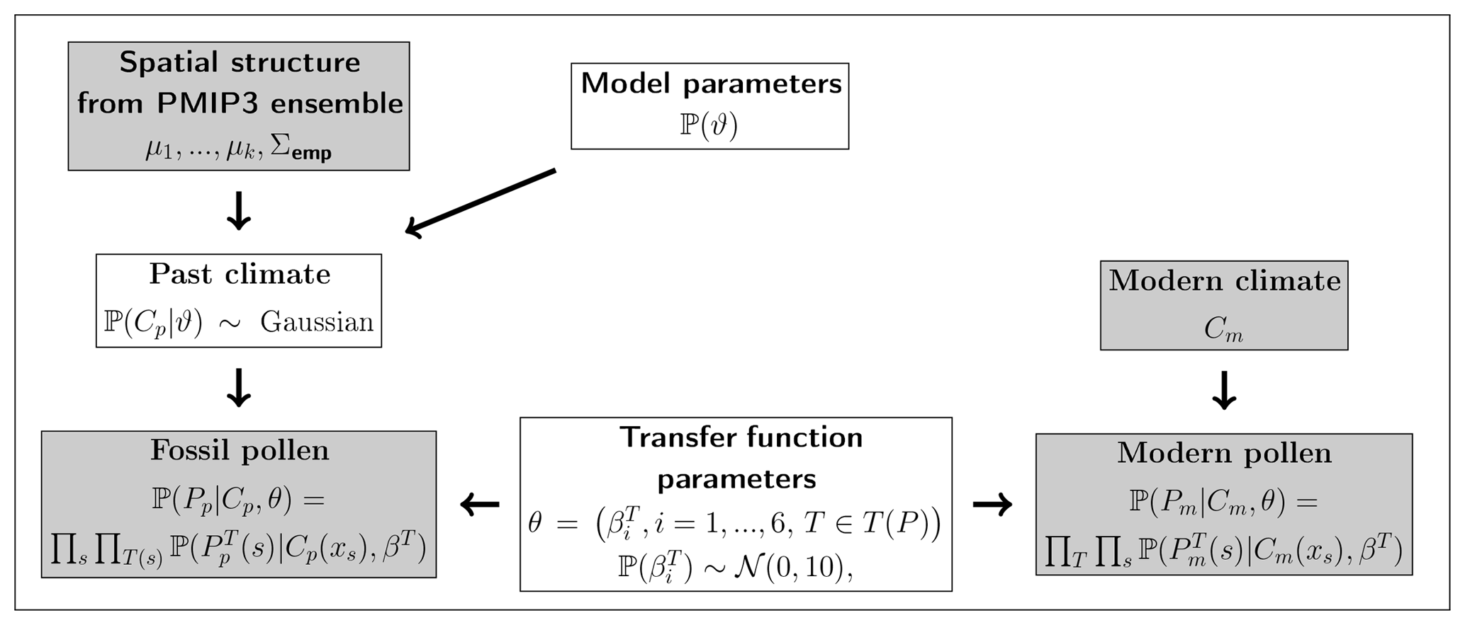
In the following, we denote fossil pollen and macrofossil data by Pp, past climate by Cp, modern vegetation and climate data for the calibration of transfer functions by Pm and Cm, respectively, and additional model parameters by Θ. We are interested in the conditional distribution of Cp and Θ given Pp, Pm, and Cm; i.e., we want to estimate the posterior distribution . Applying Bayes' theorem to (in the following, we omit normalizing constants), we get
Following Tingley and Huybers (2010), we call the data stage, the process stage, and ℙ (Θ) the prior stage. In paleoclimatology, the data stage is traditionally called a transfer function, which in our case is formulated in a forward way. It probabilistically models the proxy data given climate variables and is described in detail in Sect. 3.2. The process stage stochastically interpolates the local climate information from the proxy data to a spatial domain and is described in Sect. 3.3. The prior stage defines prior distributions for the model parameters Θ, which are necessary to ensure that the posterior is a valid probability distribution (Gelman et al., 2013).
To further structure the framework, we split the model parameters Θ into θ, which represents parameters associated with the data stage, and ϑ, which represents parameters that influence the process stage. We assume that θ and ϑ are a priori independent of each other and that the data stage is conditionally independent of ϑ given Cp. Furthermore, by construction, Pm and Cm only contribute to the reconstruction via the transfer function parameters; i.e., they are assumed to be independent of all other quantities. Hence, we can rewrite Eq. (1) and get
Here, is called the calibration stage and is called the observation stage (Parnell et al., 2015). The structure of the Bayesian model can be expressed by a directed acyclic graph as shown in Fig. 2.
3.2 Transfer function
The Bayesian model uses probabilistic transfer functions to model proxy data, in our case occurrence information on taxa, given a climate state and transfer function parameters. From all the terms in Eq. (2), the calibration stage, the observation stage, and the prior distribution of the transfer function parameters are related to the transfer function. As described above, our main reconstruction target is the bivariate climate , where C1 is MTWA and C2 is MTCO.
To reconstruct climate from the Simonis et al. (2012) synthesis, the probabilistic indicator taxa method (PITM) is used, which is a well-established transfer function to quantitatively constrain past climate states with occurrence information on taxa. It uses taxa that are sensitive to MTWA and MTCO and determines the climatic niche where they occur by fitting response functions. The classical indicator taxa method (Iversen, 1944) estimates binary limits. PITM, also called the probability density function (PDF) method in the literature (Kühl et al., 2002), is an extension wherein probability distributions are fitted to acknowledge the fact that the transitions between climates in which taxa usually occur and those in which they do not grow are soft. Initially, Gaussian distributions were used for calibration (Kühl et al., 2002) against vegetation maps (Schölzel et al., 2002). Later, the model was extended to mixtures of Gaussians (Gebhardt et al., 2008) and quadratic logistic regression (Stolzenberger, 2011, 2017).
We integrate the forward formulation of PITM from Stolzenberger (2017) in our Bayesian framework. For each taxon, we fit a quadratic logistic regression model describing the probability of taxa occurrence for a given value of C. The idea of using quadratic logistic regression stems from the BIOMOD software for predicting species distributions (Thuiller, 2003). The regression for taxa T contains linear and quadratic terms for each of the climate variables as well as an interaction term:
Here, “logit” denotes the logistic function, and , …, represents regression coefficients. This regression leads to a unimodal response function that is anisotropic but has two symmetry axes, as can be seen for dwarf birch (Betula nana) and European ivy (Hedera helix) in Fig. 3.
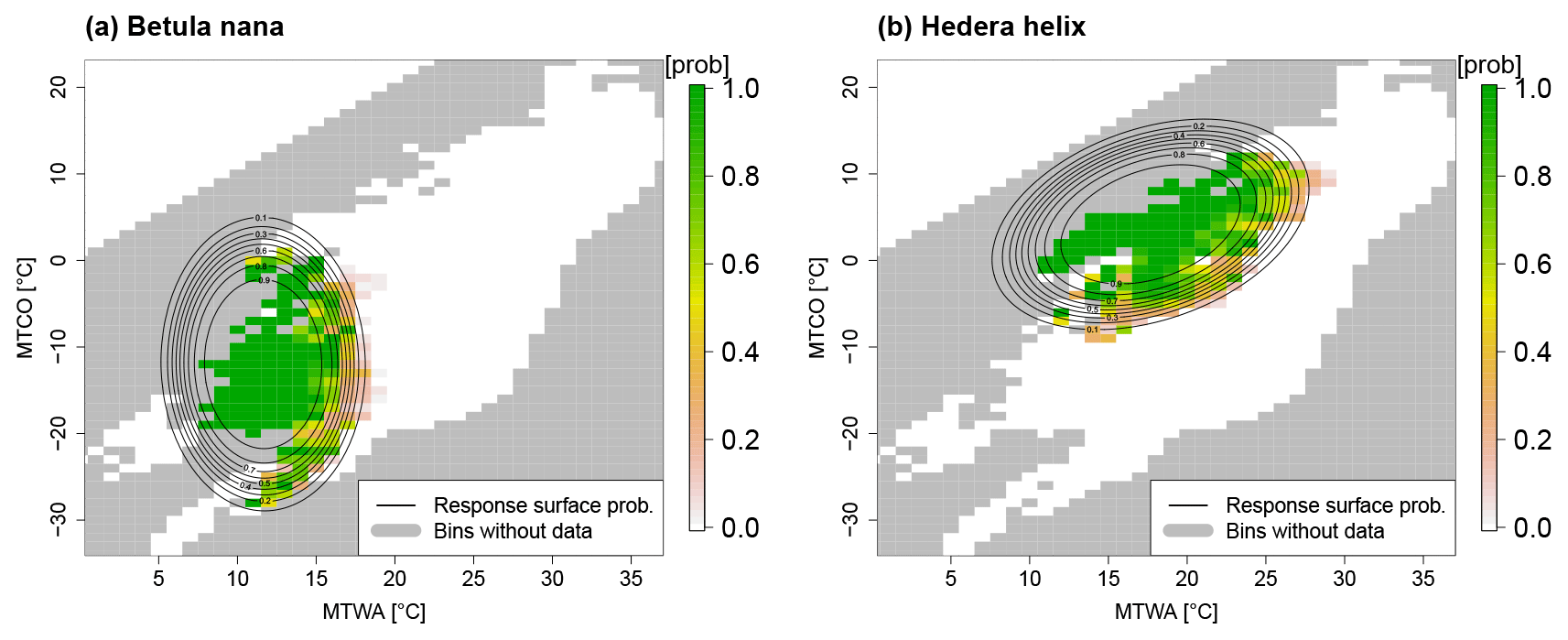
Figure 3Response functions for (a) Betula nana and (b) Hedera helix. The relative frequency of occurrence in 1 K bins is shown in colors, and the contours depict the probability of presence as estimated by the logistic response function. Gray boxes denote bins without calibration data. In the climate space, combinations of MTWA and MTCO with MTWA < MTCO cannot occur by definition. White bins in the upper left depict artificial absence information added to account for this constraint.
To fit response functions, vegetation data are used because they contain more accurate information on the occurrence of a taxon on the spatial scales of interest compared to modern pollen samples. The disadvantage of using vegetation data for the calibration is that the probability of the presence of a taxon is only valid in vegetation space on the spatial scale taken for the training data but not in the pollen or macrofossil space in which there can be multiple non-climatic reasons for the absence of a taxon like local plant competition or pollen transport effects, as well as local climatic effects below the resolution of our reconstruction.
For the calibration against the modern dataset, we use presence (T=1) as well as absence (T=0) information on the taxa that is justified by assuming that the vegetation maps contain accurate information on taxa presence and absence. From the definition given in Sect. 2.3, it follows that at any location MTWA is larger than or equal to MTCO. Formally incorporating this constraint into the inference leads to a nonlinear condition on the regression parameters, which is very hard to implement. Therefore, we choose the more practical way of adding artificial absence information for combinations of MTWA and MTCO such that MTCO > MTWA. This makes reconstructions of MTCO values larger than MTWA very improbable. To apply the response functions for individual taxa to a set of proxy data, we assume that proxy samples P(s), where s=1, …, S subscripts the proxy samples, are conditionally independent given a climate field and that, conditioned on C(xs), where xs is the location of the sth sample, P(s) is independent of the climate at all other locations. This leads to the following probabilistic model for the set of modern vegetation samples:
Here, is the presence or absence of taxa T in the sth calibration sample, T(P) is the set of all taxa occurring in the fossil pollen and macrofossil synthesis, and .
As described above, the absence of a taxon in a pollen or macrofossil sample can have reasons that are not included in the absence probability estimated from Eq. (4), as this calibration is only valid in the vegetation space. As information on the absence of a taxon in the vegetation space is not available from pollen and macrofossil data, the only reliable occurrence information on a taxon in the respective grid box in the past is the presence of the taxon in a pollen or macrofossil sample (Gebhardt et al., 2003). Hence, only occurring taxa are included in the reconstruction step. Violations of the assumption that taxa are treated as conditionally independent given climate, i.e., due to the co-occurrence of taxa (Kühl et al., 2002), can lead to over-fitting. Therefore, a statistical preselection of taxa, which are present in a sample, is applied (Gebhardt et al., 2008). For the pollen and macrofossil synthesis used in this study, the preselection was carried out by Simonis (2009) and we follow his results. Following these considerations, is given by
where T(s) represents the taxa occurring in sample s and picked by the preselection procedure.
Finally, we define a prior distribution for θ. We use a Gaussian distribution centered at 0 and a marginal variance of 10 for each parameter . Due to the absence of prior information on the correlation structure, we assume independence between the taxa as well as within a taxon. Due to the high information content in the calibration dataset, the influence of the prior on the response functions is negligible for most taxa. It slightly smooths the corresponding maximum likelihood estimates, particularly for rare taxa, but does not influence the reconstructions significantly.
Using a flat prior for Cp(xs) and removing spatial correlations, local climate reconstructions at the locations of the proxy samples can be calculated. These reconstructions depend only on the proxy data in grid box xs. Results of local MH reconstructions for each grid box with proxy data are shown in Fig. 4, where the local reconstruction means and 90 % credible intervals (CIs) are plotted. Local reconstructions can also be used to evaluate the ability of the transfer functions to reconstruct modern climate, which provides a reference for possible regional biases. For the PITM model such evaluations have been performed by Gebhardt et al. (2008) and Stolzenberger (2011). Both evaluations show that the model tends to underestimate north–south gradients, leading to positive biases in Fennoscandia and slightly negative biases in the Mediterranean. The biases and the uncertainties are larger for winter temperature than for summer. Therefore, results for MTCO in northern Fennoscandia should be treated with caution, while for all other regions the biases of the reconstruction means are within reconstruction uncertainties.
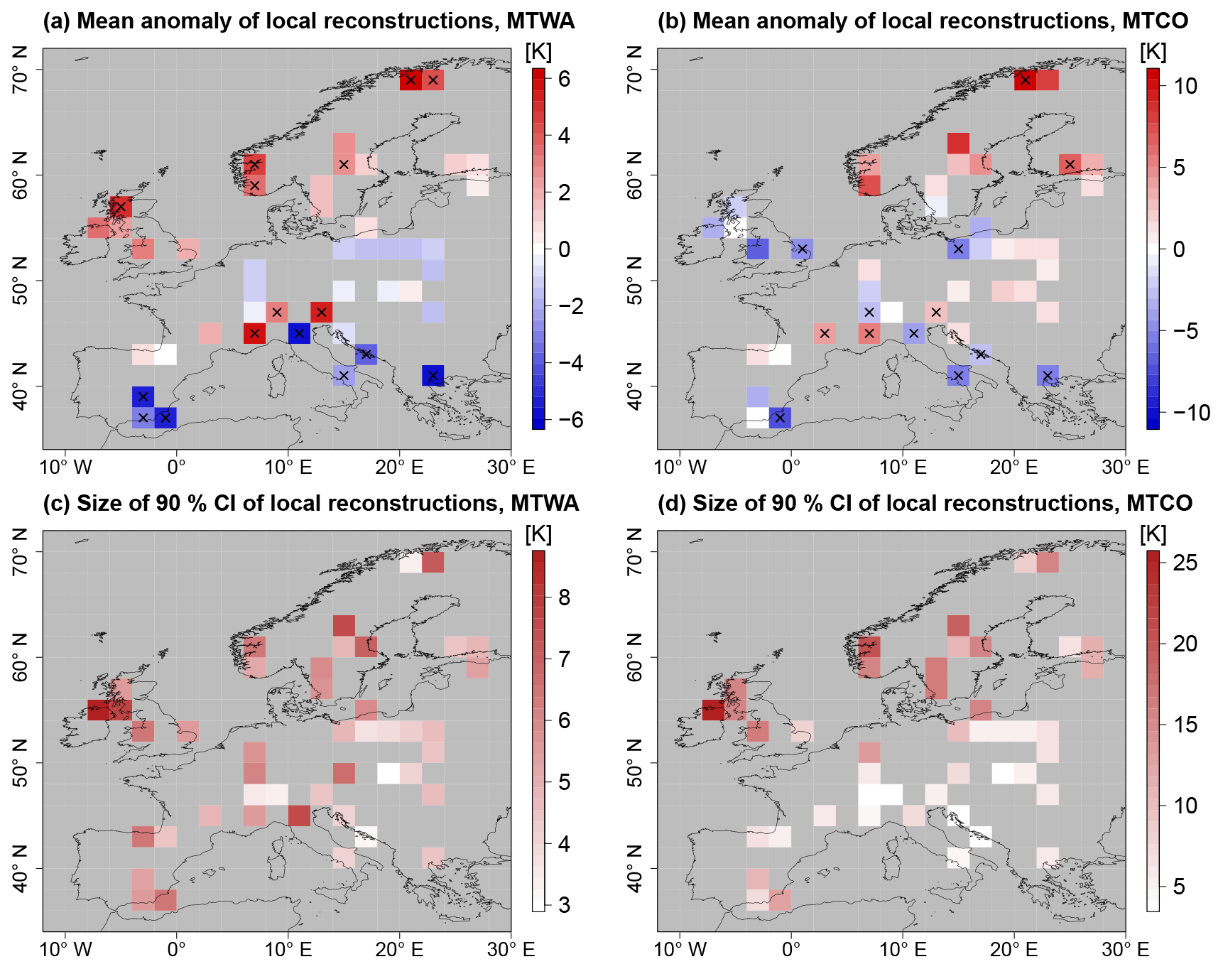
Figure 4Summary statistics of local reconstructions using the PITM forward model. (a, b) Mean anomaly from CRU reference climatology; significant anomalies (5 % level) are marked by black crosses. (c, d) Uncertainty measured by the size of marginal 90 % CIs.
An issue of the PITM version used in this study is the inconsistent use of calibration and fossil data by using presence and absence information on taxa for the calibration but only occurring taxa in the reconstruction. Despite this inconsistency, the reconstructions in this study are in agreement with previous versions of PITM, for which only occurrence information was used for calibration. However, there is no simple solution for the problem that the calibration is in vegetation space, whereas the absence of taxa in the fossil samples is information in the pollen or macrofossil space. A promising idea might be to model the absence due to non-climatic reasons as zero inflation by adding a latent variable to estimate the detection probability of a taxon (MacKenzie et al., 2002). But the estimation of detection probabilities is a very challenging task because it depends on many factors like pollen influx area, local topography, soil properties, and plant competition, which might change over time. In addition, the processes that influence the detection probability of macrofossils are very different than for pollen. Therefore, a different detection probability has to be estimated for pollen than for macrofossils. Resolving the described issues is an interesting direction for future research but is beyond the scope of this study.
3.3 Process stage
The ensemble of climate simulations is used to control the spatial structures of the reconstruction and to constrain the range of physically possible climate states for a given external forcing by computing a spatial prior distribution from the ensemble members. This distribution is combined with interpolation parameters ϑ to facilitate a more flexible adjustment to the proxy data. The estimation of the prior distribution is hampered by the small number of ensemble members K=7.
It is not obvious which method for estimating the prior distribution is best suited for the problem at hand and which additional model parameters are appropriate to preserve as much physical consistency contained in the climate simulations as possible but to correct for climate model inadequacies. Therefore, we perform a comparison study of six process stage models that are composed of three techniques to formulate the process stage and two choices for the involved spatial covariance matrix.
3.3.1 Gaussian model
The most common approach in the data assimilation literature is to assume that the ensemble members are independent and identically distributed (iid) samples from an unknown Gaussian distribution of possible climate states (Carrassi et al., 2018). In the following, the climatological means of the K ensemble members are denoted by μk. Subsequently the spatial prior distribution is given by , where 𝒩 denotes a Gaussian distribution, is the ensemble mean, and Σprior is a spatial covariance matrix, which is given by a regularized version of the empirical covariance:
The superscript t denotes the matrix transpose. Hence, the covariance matrix is based on the inter-model differences as an estimate of epistemic uncertainties. The regularization techniques of Σemp are specified below. The Gaussian distribution is N-dimensional, where N is the number of grid boxes times the number of jointly reconstructed variables.
The main advantage of this Gaussian model (GM) is that inference is simpler than in more complex probability density estimation techniques. The disadvantage is that it relies on the strong assumption that μk represents iid samples from an unknown Gaussian distribution. This assumption tends to be more realistic for samples from just one ESM, whereas statistics of multi-model ensembles are often not well described by purely Gaussian distributions (Knutti et al., 2010). A second disadvantage of this model is that the absence of additional parameters limits the possibilities to adjust the posterior distribution to the proxy data. The third disadvantage is that the spatial structures of individual ensemble members are lost by averaging over all members. Nevertheless, in many climate prediction applications multi-model averages outperformed each individual ESM (e.g., Krishnamurti et al., 1999).
3.3.2 Regression model
A relaxation of the assumptions of the GM is the second model, which we call the regression model (RM) because it is inspired by regression-based models popular in postprocessing and climate change detection and attribution (Hegerl and Zwiers, 2011). In the RM, variable weights λk, k=1, …, K are introduced to allow for weighted averages of the ensemble members. This means that samples that fit better to the proxy data are weighted higher in the posterior. The sum of the weights is set to one such that an unrealistically warm or cold state is prevented. This leads to the process stage model
and an additional prior distribution for the model weights,
“Dir” denotes a Dirichlet distribution, which guarantees that the weights take values between zero and one and sum up to one. Conditioned on λ, the process stage distribution is Gaussian, but non-Gaussianity is permitted through the variable weights. The parameters of the prior distribution are chosen to prefer combinations with one dominant ensemble member that is adjusted by the other members to improve the fit to the proxy data. Thereby, it preserves more physical structures from individual members than the GM, as better-fitting models are only weakly corrected for climate model inadequacies. The RM has the advantage of possessing more degrees of freedom compared to the GM. The inference process becomes a little more involved than for the GM because the ensemble member weights have to be estimated, too, but the conditional Gaussian distribution of Cp helps design efficient inference algorithms.
3.3.3 Kernel model
The third model has been introduced in the data assimilation literature by Anderson and Anderson (1999) to combine particle and Gaussian filtering approaches. This kernel model (KM) assumes that each ensemble member is a sample from an unknown distribution of possible climate states given a set of forcings, but it does not assume that this unknown distribution is Gaussian. Instead, nonparametric kernel density estimation techniques (Silverman, 1986), in which the probability distribution is given by a mixture of multivariate Gaussian kernels, are used. Each ensemble member climatology corresponds to the mean of a kernel.
Ideally, the covariance matrix of each kernel would correspond to the respective ESM such that the spatial autocorrelation of that ESM is preserved when we sample from its kernel. Unfortunately, there is only one MH run available for each ESM, and the internal variability in those runs is much smaller than the inter-model differences. Using the internal variability of those runs would thus lead to very distinct kernels and allow for too few climate states. Therefore, the covariance of each kernel is estimated from the inter-model differences even though autocorrelation of the individual models is lost. This is a very common choice in kernel-based probability density approximations (Liu et al., 2016; Silverman, 1986).
Compared to the GM, the empirical covariance matrix Σemp is scaled by the Silverman factor (Silverman, 1986),
which optimizes the variances of the kernels. Hence, in the KM the scaled empirical covariance matrix , given by , is regularized, leading to the spatial covariance matrix . Note that the small number of ensemble members leads to a standard deviation reduction of only around 2 % in our applications.
Each kernel gets an assigned weight ωk, k=1, …, K, which is inferred in the Bayesian framework. The weights sum up to one. The resulting process stage is a mixture distribution:
A Dirichlet distributed prior is used for ω with parameter for each of the K components. A computational disadvantage of the KM is that the process stage is multi-modal and non-Gaussian. We augment the model with an additional parameter z, which follows a categorical distribution, denoted by “Cat”, to restore Cp as Gaussian conditioned on ω and z. z selects a kernel k according to its weight ωk, i.e., z is defined such that
Integrating out z yields the mixture distribution Eq. (10).
Two advantages of the KM are that it is not assumed that the unknown prior distribution is Gaussian and that the kernels do not rely on an iid assumption for their first-moment properties. However, the KM still relies on an iid assumption for the second moments. The KM preserves the spatial structures of each ESM in the first moments of the kernels. This preservation of physical consistency reduces the degrees of freedom compared to the RM. For example, when the true climate state lies exactly between μ1 and μ2, the posterior mode cannot be changed to , which is possible in the RM. Another disadvantage of the KM is that the multi-modality makes the design of efficient inference algorithms a lot more challenging.
3.3.4 Glasso-based covariance matrices
The first technique to regularize the empirical covariance matrix (the scaled empirical covariance in the KM), which is applied in this study, is the graphical lasso algorithm (glasso; Friedman et al., 2008, implemented in the R package glasso). This algorithm approximates the precision matrix (inverse covariance) by a positive definite, symmetric, and sparse matrix . Therefore, Σprior is a valid N-dimensional covariance matrix. Glasso maximizes the penalized log likelihood:
where ξ is the penalty parameter, is the vector L1 norm, and the first two terms are the Gaussian log likelihood. Because applying the glasso algorithm is computationally expensive, it is not feasible to formally include ξ in the Bayesian framework. Instead a suitable value of ξ has to be determined prior to the inference. In this study, ξ is chosen such that Σprior is a numerically stable covariance matrix and the performance in cross-validation experiments (CVEs) is optimized. Technical details on the determination of ξ are described in Appendix A.
The advantage of the glasso approach is that the empirical matrix can be approximated very closely and the sparseness of the precision matrix facilitates the use of efficient Gaussian Markov random field (GMRF) techniques (Rue and Held, 2005) in the inference algorithm. A disadvantage is that no new spatial structures are added to Σemp. Therefore, the effective number of spatial modes is much smaller than the dimension of the climate vector, which can lead to a collapse onto a very small subspace of the N-dimensional state space and subsequently biases and under-dispersion.
3.3.5 Shrinkage-based covariance matrices
To overcome the deficiencies of the glasso approach, we propose an alternative covariance regularization technique. The so-called shrinkage approach (Hannart and Naveau, 2014) uses a weighted average of the empirical correlation matrix and a reference correlation matrix, which in our case contains additional spatial modes such that the effective number of spatial modes in the covariance matrix is increased. This allows for deviations from the spatial structures prescribed by the climate simulation ensemble and is therefore a strategy to account for climate model inadequacies.
Let Ψemp be the empirical correlation matrix of the climate simulation ensemble, which is related to Σemp by
where Diag(Σemp) denotes a diagonal matrix with the same diagonal entries as Σemp, and the exponent means that the square root of each diagonal entry is taken. Replacing Ψemp by a weighted average of Ψemp and a shrinkage target Φ leads to the shrinkage covariance matrix
α is the weighting parameter, which takes values between zero and one. Φ is computed from a numerically efficient GMRF approximation of a stationary Matérn correlation matrix (Lindgren et al., 2011). The Matérn correlation matrix is controlled by three parameters: the smoothness, the range ρ, and the anisotropy ν. We fix the smoothness for computational reasons. ρ controls the decorrelation length, and ν parameterizes the ratio of the meridional versus zonal decorrelation length. For joint reconstructions of multiple climate variables, independent correlation matrices for each variable are combined in a block structure. Details about the definition of Φ are given in Appendix B.
Ideally, the parameters α, ρ, and ν are estimated from the proxy data. But initial tests showed that the signal in the proxy data is not informative enough to constrain the parameters. Therefore, an ensemble of parameter combinations is created from fitting the shrinkage model to each of the climate simulation ensemble members given all other members. This results in seven consistent sets of α, ρ, and ν. Those are passed to the reconstruction framework such that each parameter set is chosen with a probability inferred from the proxy data. Thereby, each set is based on a fit against physically consistent structures, and the problem of non-identifiability of the parameters from proxy data alone is reduced. The resulting parameter estimates cover a wide range of possible values. The main advantage of the shrinkage approach over the glasso-based matrices is that more spatial modes are included in the covariance matrix. Thereby, the collapsing of the reconstruction towards a very low-dimensional subspace is mitigated.
3.4 Inference strategy
Because PITM is non-Gaussian and nonlinear, the posterior climate does not belong to a standard probability distribution. Therefore, Markov chain Monte Carlo (MCMC) techniques are used to asymptotically sample from the correct posterior distribution. These samples allow for analyses beyond summary statistics like means and standard deviations. A Metropolis-within-Gibbs strategy is implemented, which means that in each update of the Markov chain, we sample sequentially from the full conditional distributions (i.e., the distribution of the respective variable given all other variables) of θ, ϑ, and Cp. This strategy is chosen because for many variables the full conditional distributions follow probability distributions for which efficient sampling algorithms exist, and for the remaining variables Metropolis–Hastings updates are used for sampling.
To sample the regression parameters θ in Eqs. (3) to (5) efficiently, the data augmentation scheme of Polson et al. (2013) is used. For taxa T, the full conditional only depends on Cp, Cm, , and but not on other taxa. Therefore, we can sample independently from the other taxa. Polson et al. (2013) introduce help variables , l=1, …, L(T), where L(T) is the number of observations of taxa T, such that is Pólya–gamma (PG) distributed, and is Gaussian. Therefore, the MCMC algorithm samples alternately from a PG distribution using the sampler of Windle et al. (2014) and from a Gaussian distribution. The PG sampler is implemented in the R package BayesLogit (Windle et al., 2013).
Sampling from ϑ depends on the particular process stage model. In models with a shrinkage covariance matrix, α, ρ, and ν are sampled from the K parameter sets in a Metropolis–Hastings step. The weights λ in the RM are sampled from a random-walk-type Metropolis–Hastings update. In the KM, Eqs. (11) to (13) lead to full conditionals for ω and z, which are again Dirichlet and categorically distributed but with updated parameters. Therefore, Gibbs sampling can be used to update ω and z.
To sample from the full conditional of Cp, we separate the grid boxes xP with at least one proxy record from those without any proxy records denoted by xQ. There is no closed form available for the full conditionals of Cp(xP). Therefore, we use a random walk Metropolis–Hastings algorithm to update Cp(xP) sequentially for all members of xP. As the transfer functions act locally, Cp(xQ) is conditionally independent of Pp given Cp(xP) and ϑ. Therefore, we update Cp(xQ) by sampling from , which is Gaussian.
The multi-modality of the KM makes inference for this model a lot more challenging than for the GM and RM. The problem of efficient MCMC algorithms for multi-modal posterior distributions is a widely acknowledged issue in the literature (Tawn and Roberts, 2018), and in this study Metropolis coupled Markov chain Monte Carlo (MC3; Geyer, 1991), which is also known as parallel tempering, is used to overcome this issue. Details on this procedure are provided in Appendix D.
To speed up the inference, grid boxes with proxy data and those without proxy data are treated sequentially. First, Cp(xQ) is integrated out to get an estimate of the joint distribution of Θ and Cp(xP). In a second step, we sample from Cp(xQ) conditioned on Cp(xP) and Θ. The remaining bottleneck in computation time is the estimation of the transfer function parameters due to the large modern calibration set. While in theory the observation layer influences the updates of θ, in practice the influence of Eq. (5) on the posterior of θ is negligible. Therefore, a modularization approach (Liu et al., 2009; Parnell et al., 2015) is used in CVEs, wherein a sequence of reconstructions with slightly changed proxy networks is computed. This means that first MCMC samples of θ are drawn using only Eq. (4). Then, Cp is reconstructed using these samples instead of sampling θ from its full conditional.
Detailed formulas for the full conditional distributions are given in Appendix C. The pseudo-code for the MCMC and MC3 algorithms is provided in the Supplement. For a 798-dimensional climate posterior, as is the case in joint reconstructions of MTWA and MTCO with 45 grid boxes that contain at least one proxy record, 75 000 MCMC samples are created. The first 25 000 samples are discarded as burn-in. To reduce the autocorrelation of subsequent samples, every fifth sample is extracted to create a set of 10 000 posterior samples for further analyses. On a standard desktop computer, reconstructions with the modularized model are computed in approximately 30 min. The convergence of all MCMC variables is checked using the Gelman–Rubin–Brooks criterion (Brooks and Gelman, 1998) implemented in the R package coda (Plummer et al., 2006).
In this section, results from a comparison study of the six different process stage models are shown. Then, the MH reconstruction for Europe with the Simonis et al. (2012) synthesis and the PMIP3 MH ensemble is presented.
4.1 Comparison of different process stage frameworks
In this section, the reconstruction skill of the three process stage formulations (GM, RM, KM) and the two covariance models (glasso, shrinkage) are compared using two types of experiments. Identical twin experiments (ITEs) use the climate simulation ensemble by simulating pseudo-proxy data from one ESM and trying to reconstruct that reference climatology from the simulated proxies and the remaining ensemble members. These experiments facilitate the understanding of different modeling approaches for the process stage in a controlled environment. In particular, the evaluations do not have to rely on indirect observations, as is the case in real paleoclimate applications for which the true climate state is unknown. The second type of experiments are CVEs for which spatial reconstructions with the Simonis et al. (2012) synthesis are performed but the samples from one grid box are left out. Then, the reconstructions for this grid box are evaluated against the left-out sample in the vegetation space. The advantage of these experiments is that the models are compared in a real-world setting. The disadvantage of CVEs is that no direct observations of paleoclimate are available such that evaluations against observations have to be indirect.
4.1.1 Identical twin experiments
The first step in an ITE is to choose a reference ESM with climate state . Then, for each grid box that contains samples from the Simonis et al. (2012) synthesis (denoted by xP), pseudo-proxies are simulated from a Gaussian approximation of the uncertainty structure of the local reconstructions depicted in Fig. 4. The pseudo-proxies are assumed to be unbiased with a bivariate Gaussian distribution and covariance matrix , i.e.,
Using unbiased Gaussian pseudo-proxies is a common strategy to test climate field reconstruction techniques (e.g., Gomez-Navarro et al., 2015). It allows for a direct study of the ability of the process stage methods to estimate spatial climate fields from sparse and noisy proxy data, without having to factor in potential biases in the transfer function. Finally, a probabilistic spatial reconstruction is computed from the simulated proxies and the remaining ensemble members. For each of the six different process stage configurations and each of the seven PMIP3 ensemble members as reference climatology, five randomized ITEs are performed. The evaluation of the ITEs focuses on biases in the reconstructions, potential under-dispersion, and the ability of the reconstruction to probabilistically predict past climate.
Averaged over all ITEs with the same process stage model and averaged in space, the mean deviation between the reference climate and posterior mean as a measure for systematic biases is close to 0 K for all process stage models with values between −0.14 K for the shrinkage KM and +0.03 K for the shrinkage RM (Table 2, Fig. 5a), but the variation across ITEs is larger for the glasso covariance models (standard deviation around 0.31 K) than for the shrinkage covariance models (standard deviation around 0.24 K). The standard deviations for MTCO reconstructions tend to be larger than for MTWA. This can be explained by the larger noise level in the local MTCO reconstructions, which makes the spatial MTCO reconstructions more susceptible to biases. Concerning the spatial patterns of mean deviations, all ITEs with glasso covariance matrices exhibit larger local biases than those with shrinkage matrices (see additional figures in the Supplement). While the magnitude of biases for the GM and RM models with shrinkage covariances is much smaller, the magnitude of local deviations of the shrinkage KM is just slightly smaller than for glasso covariances. This shows that the models with a shrinkage matrix can reconstruct spatial patterns better than the models that use glasso. In addition, averaging over different ensemble members in the process stage mean seems to be a more effective strategy as the GM and RM reconstruct the spatial structures better than the KM.
Table 2Summary measures for ITEs and CVEs. Summary measures for ITEs and CVEs with the six process stage models.
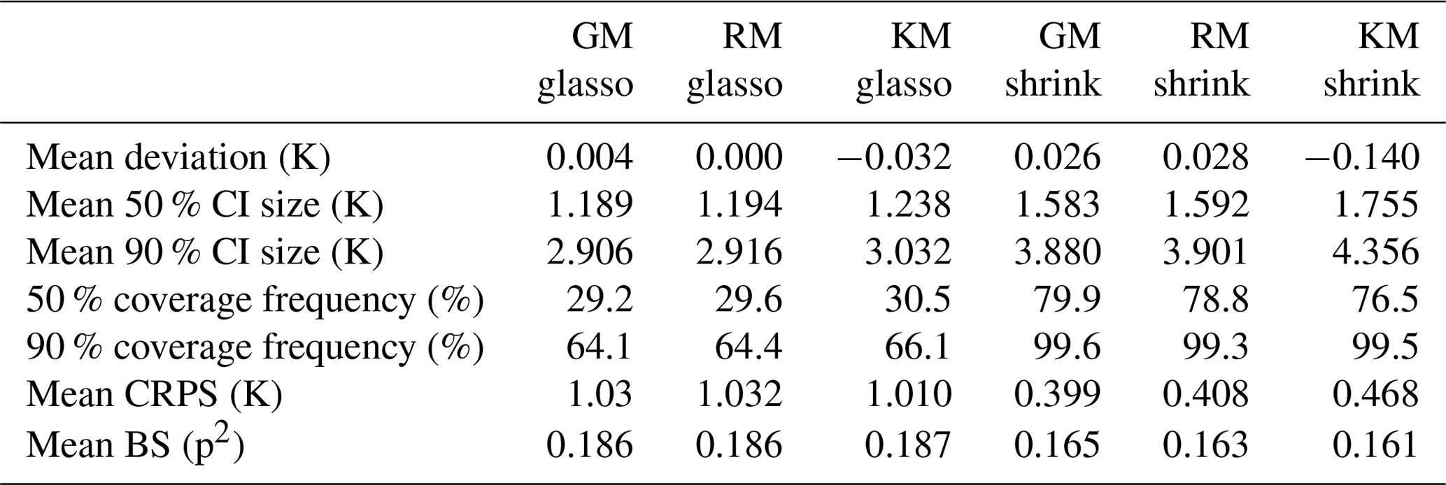
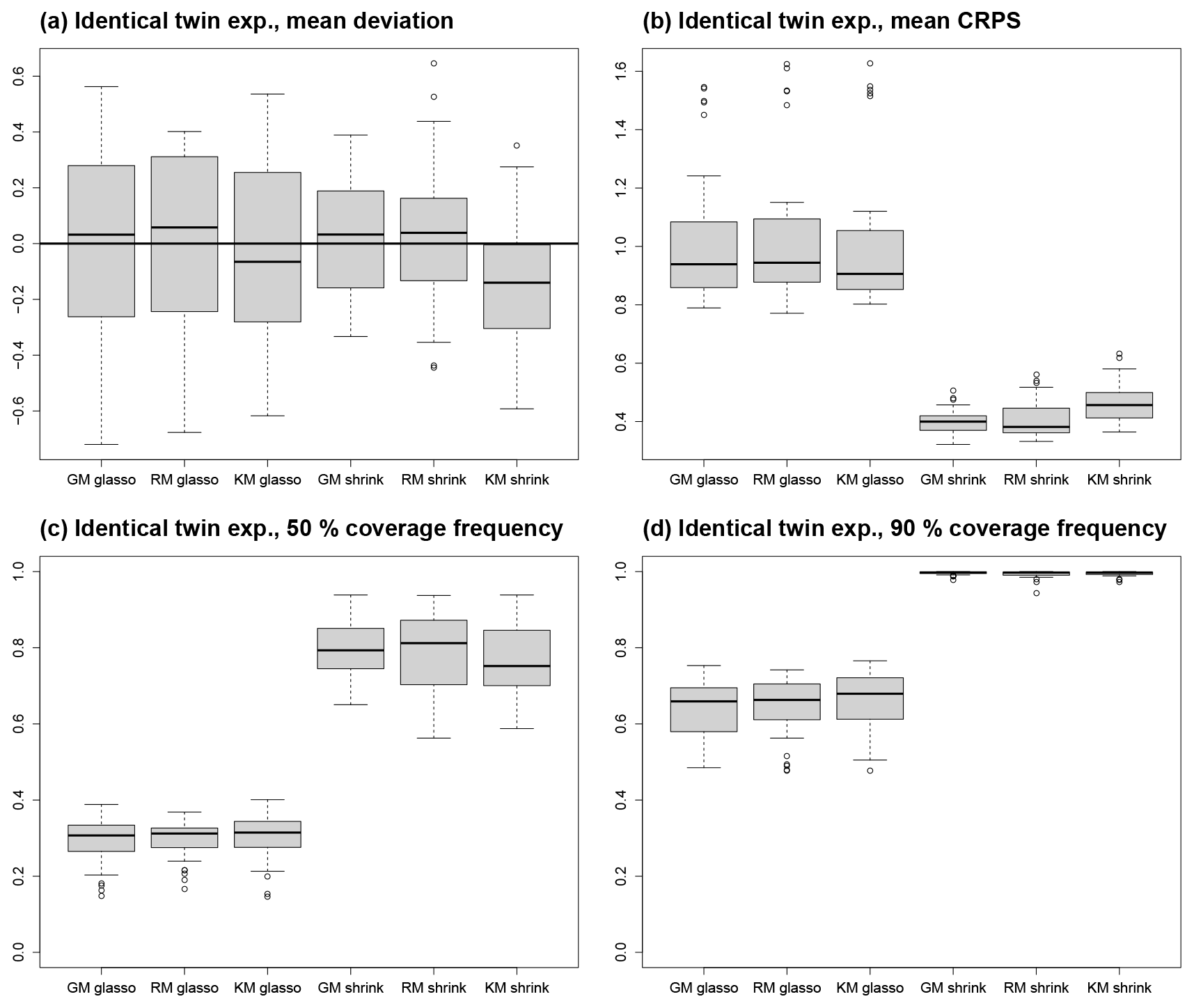
Figure 5Results from ITEs. The box plots depict the distribution of experiments with the same process stage model. (a) Mean deviation from reference climate, (b) mean CRPS, (c) coverage frequency of 50 % CIs, and (d) coverage frequency of 90 % CIs.
The higher number of spatial modes in the shrinkage covariances leads to larger posterior uncertainties than for the glasso models because the limited information contained in the proxy data can constrain only a small number of spatial modes (Table 2). To study the dispersiveness of the reconstruction, coverage frequencies for 50 % and 90 % CIs are calculated. This means that the frequency of the reference climate state to be included in the respective CIs is computed. For the 50 % CIs, coverage frequencies below 50 % indicate under-dispersiveness, whereas values above 50 % indicate over-dispersion. Similarly, the target for the 90 % CIs is 90 %. In all ITEs, the glasso models are under-dispersive, and the shrinkage models are over-dispersive (Table 2, Fig. 5c). The coverage frequency for 50 % CIs is below 41 % in all ITEs with a glasso covariance matrix and above 56 % in all ITEs with a shrinkage covariance matrix. Similarly, the coverage frequencies for 90 % CIs are below 77 % for all glasso ITEs and above 94 % for all ITEs with a shrinkage matrix (Fig. 5d). In most grid boxes of the ITEs with a glasso-based covariance matrix, the coverage frequencies are below the target values, whereas they are above the desired values in almost all grid boxes in the ITEs with a shrinkage matrix (see additional figures in the Supplement). The values are closest to the target near grid boxes with proxy data in all ITEs.
To analyze the combined effect of biases and dispersiveness, the continuous ranked probability score (CRPS) is computed. This is a common strictly proper score function for evaluating probabilistic predictions (Gneiting and Raftery, 2007), in our case the ability of a reconstruction method to probabilistically predict past climate from sparse and noisy data. It is a generalization of the absolute error to probabilistic forecasts (Matheson and Winkler, 1976) given by
where F is the cumulative distribution function of the reconstruction Cp at grid box x, and is the reference climate state at x. The CRPS has a unique minimum at 0 and is positive unless F is a perfect prediction.
With a spatially averaged mean around 1 K for all three models, the ITEs with glasso covariance matrices feature a higher CRPS than the ITEs with shrinkage matrices that have a spatially averaged mean around 0.4 K (Table 2, Fig. 5b). This is a result of larger biases on the grid box level and under-dispersiveness of the posterior distribution. In addition, the variability between the ITEs with the same process stage model is higher for models with glasso covariance, which shows that these models are less robust. The MTWA CRPS is slightly lower than the MTCO CRPS since the local reconstructions constrain MTWA more than MTCO. Among the process stage models with a shrinkage matrix, the KM performs slightly worse than the GM and the RM as a result of the larger biases on the grid box level described above. The spatial structures of CRPS reflect the mean deviation patterns (Fig. 6). This is an effect of more pronounced spatial patterns in the mean deviations compared to dispersiveness.
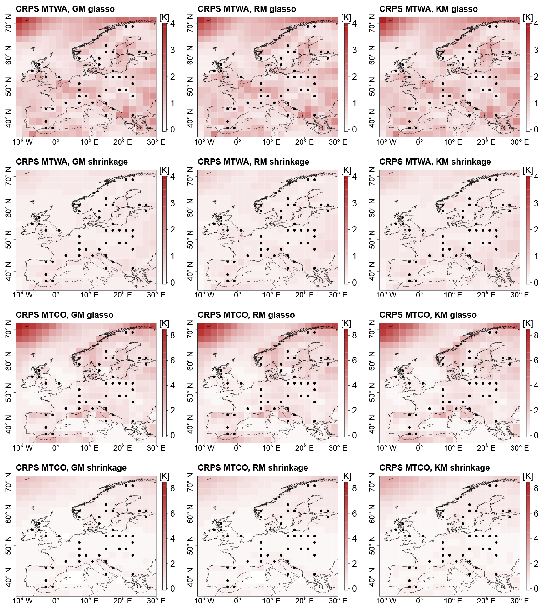
Figure 6Mean CRPS in ITEs for GM, RM, and KM. Top row: models with glasso covariance matrix, MTWA. Second row: models with shrinkage covariance matrix, MTWA. Third row: models with glasso covariance matrix, MTCO. Bottom row: models with shrinkage covariance matrix, MTCO. Grid boxes with simulated proxy data are depicted by black dots.
4.1.2 Cross-validation experiments
CVEs are a way to understand the ability of a spatial reconstruction method to produce consistent estimates. In paleoclimatology, the issue is that all observations are indirect, which means that poor evaluations can result from errors in the process stage or the data stage. The assumption behind CVEs is that the data stage is unbiased or at least consistently biased among different proxy samples. Cross-validations are evaluated in the observation space. In this study, this is the vegetation space, i.e., the occurrence of taxa in a grid box. As the only reliable information available from the pollen and macrofossil synthesis on the vegetation composition in a grid box is the presence of certain taxa, this is also the only data used for the evaluation. Due to the sparseness of the proxy network, leave-one-out CVEs are performed and no more data are left out in each experiment.
In each CVE, a reconstruction with the Bayesian framework is computed with all proxy samples except for those in one grid box x. Then, the reconstruction Cp(x) at grid box x is extracted and treated as a probabilistic prediction of the climate at x. Next, the PITM forward model is applied to C(x) for each sample Pp located in grid box x to produce probabilistic predictions of the occurrence of the taxa that are found in those samples. This prediction of the occurrence of a taxon T is represented by the probability of presence . A common score function for binary variables is the Brier score (BS; Brier, 1950) given by
where δT denotes the indicator function of taxa T. The BS takes values between zero and one; zero corresponds to a perfect prediction and one to the worst possible prediction. The PITM forward model is applied to each MCMC sample, which leads to a set of probabilistic predictions pj(T), j=1, …, J for taxa T. Predictions are calculated for each taxon that occurs in sample P(s). The joint score of P(s) is then calculated by averaging the BS of each taxon and prediction:
If multiple samples are assigned to one grid box, the mean score of those samples is taken.
A problematic step in the methodology described above is that the BS is only evaluated for occurring taxa for the reasons discussed in Sect. 3.2. This can make the BS improper when comparing statistical models that predict the presence or absence of taxa. However, the goal of the methodology described above is an indirect evaluation of predictions of past climate via transfer functions. In that context, it would lead to inconsistencies between the local reconstructions and the BS evaluations if taxa that are absent in the proxy synthesis were included. Circumventing this issue is beyond the scope of this study. It should be noted that for each taxon the BS is a convex function of climate and minimal for a unique climate state. These two properties make the methodology described above useful for the indirect evaluation of climate field reconstruction methods.
The models with glasso covariances perform slightly worse than those with shrinkage covariances, as the mean BS takes values of 0.186 (GM, RM) or 0.187 (KM) for the glasso-based models compared to values between 0.161 and 0.165 for models with shrinkage covariances (Table 2). Similar to the ITEs, the differences between models with different covariance types are larger than those with the same covariance model. Accordingly, the largest differences in individual grid boxes between models with different covariance matrix types are on the order of 10−1 but only on the order of 10−2 between models with the same covariance type. The models with shrinkage covariance matrices tend to perform better in western Europe and Fennoscandia, whereas in central and eastern Europe, the magnitude of the differences is very small and the models with glasso covariance matrices perform slightly better in the majority of grid boxes.
4.1.3 Conclusions from the comparison study
The ITEs show that the models with shrinkage matrix covariances are more dispersive, less biased, and more robust than those with glasso covariance matrices. These properties transfer to the CVEs in which the models with a shrinkage covariance matrix perform better, too. The results from models with the same covariance matrix are very similar except that the KM with a shrinkage covariance matrix is on average more biased than the respective GM and RM. This shows that the covariance matrix choice determines the reconstruction skill more than the general formulation of the process stage as Gaussian, regression, or kernel model. The reason for this strong effect of the regularization technique might be the small ensemble size and the fact that the modes of the inter-model variability do not explain the spatial variability of the climate optimally, which further reduces the useful spatial modes in the empirical covariance matrix.
The better performance of shrinkage covariance models shows that the low number of spatial modes is the main reason for the under-dispersiveness of the glasso-based models. On the other hand, the over-dispersiveness of the shrinkage models should be an indicator that this model is not under-dispersed even in real-world applications that face additional challenges from potentially biased or under-dispersed transfer functions and a more sophisticated spatial structure of the climate state than in the ESM climatologies. Additionally, this over-dispersiveness shows that in most regions the ensemble spread is wide enough to lead to reconstructions that do not feature posterior distributions that are too narrow.
The larger biases of the KM with the shrinkage covariance matrix compared to the GM and RM are a result of ensemble member weight degeneracy in the particle filter part of this model. The ensemble member weights tend to degenerate towards the least deviating model such that the mean values are biased towards that model. This tendency increases with the strength of the proxy data signal. This is a well-known issue of Bayesian model selection (Yang and Zhu, 2018) and therefore also of particle filter methods (Carrassi et al., 2018), which hinders the use of KMs in data assimilation problems. To mitigate this issue, the particle filter part of the KM is combined with a Gaussian part that is more similar to Kalman-type filters. The ITEs show that this adjustment is strong enough to avoid under-dispersiveness, but the degeneracy of the ensemble member weights still leads to larger biases than in the RM and GM.
4.2 Spatial reconstruction of European MH climate
Based on the results presented in the previous section, the models with a shrinkage matrix should be preferred over those with glasso covariance models. In addition, the smaller biases and more robust nature of the GM and RM with the shrinkage covariance matrix compared to the KM model makes them superior choices. Because the RM adjusts more flexibly to the proxy data than the GM, this model is presumably better suited to deal with additional caveats of real-world applications. Therefore, this model is used for the spatial reconstructions, whose results are presented in this section. Reconstruction results are summarized in Table 1. Results from reconstructions with the other five process stage models are presented in the Supplement.
4.2.1 Posterior mean and uncertainty structure
The spatially averaged mean temperature of the reconstruction (posterior mean) is 18.27 ∘C (90 % CI: (17.79 ∘C, 18.75 ∘C)) for MTWA and 1.81 ∘C (90 % CI: (1.22 ∘C, 2.45 ∘C)) for MTCO, which in both cases is warmer than the CRU reference climatology (+0.51 K for MTWA and +0.69 K for MTCO). Larger anomalies are found for subregions (Fig. 7a, b). For MTWA as well as MTCO, temperatures were cooler than today in many southern European areas, while in northern Europe the temperatures were predominantly higher than today. More specifically, MTWA was warmer over Fennoscandia, the British Islands, and the Norwegian Sea. Most of these anomalies are significant on a 5 % level. Here, a positive anomaly is called significant if the posterior probability to exceed the reference climatology is at least 0.95. Significant negative anomalies are defined accordingly. The significance estimates are calculated point-wise. Negative MTWA anomalies are found in large parts of the Mediterranean and eastern Europe, but fewer anomalies are significant on a 5 % level than in northwestern Europe. The largest positive MTCO anomalies are found in Fennoscandia and off the Norwegian coast. In the other parts of the domain, the majority of MTCO anomalies are negative, but the spatial pattern is more heterogeneous than for MTWA. A lot fewer MTCO anomalies are significant on a 5 % level compared to MTWA anomalies.
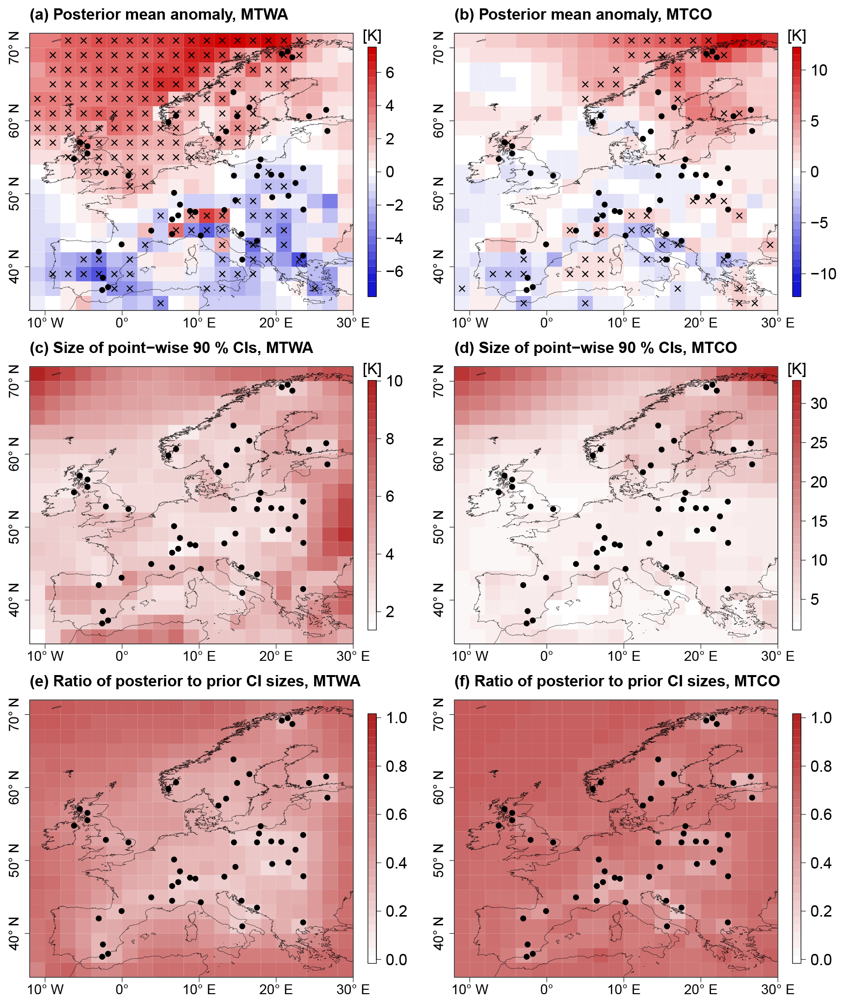
Figure 7Spatial reconstruction for MH. (a, b) Posterior mean anomaly from CRU reference climatology; point-wise significant anomalies (5 % level) are marked by black crosses. (c, d) Reconstruction uncertainty plotted as the size of point-wise 90 % CIs and (e, f) reduction of uncertainty from posterior to prior measured by the ratio of posterior to prior point-wise 90 % CI sizes. Black dots depict proxy samples.
Most of the taxa used in the reconstruction are more strongly confined for MTWA than for MTCO because the growth of most European plants is more sensitive to conditions during the growing season. This results in more constrained local MTWA reconstructions (Fig. 4c), which is in concordance with findings from Gebhardt et al. (2008). Hence, the uncertainty in the MTWA reconstruction is smaller than in the MTCO reconstruction, with spatially averaged point-wise 90 % CI sizes of 4.15 and 5.84 K, respectively (Fig. 7c, d). The uncertainty is smallest in grid boxes with proxy records and highest in the northeastern and northwestern parts of the domain where the PMIP3 ensemble spread is large and the constraint from proxy data is weak. For MTWA, additional regions with large uncertainties are found at the eastern and southern boundaries of the domain due to weak proxy data constraints.
The highest reduction of uncertainty due to the inclusion of proxy data is found in grid boxes with proxy data, as quantified by a spatially averaged reduction of point-wise CI sizes from prior to posterior of 50.1 % compared to 26.0 % for grid boxes without proxy data (Fig. 7e, f). The uncertainty reduction for MTWA is higher for terrestrial grid boxes than marine ones, but the smaller PMIP3 ensemble spread over the British Islands, the North Sea, and the Bay of Biscay leads to similar posterior CI sizes in these areas. For MTCO, the reduction of uncertainty is generally smaller than for MTWA due to the weaker proxy data constraint.
To study whether the degree of spatial smoothing of the reconstruction is reasonable, a measure inspired by discrete gradients is calculated. For each grid box, the mean absolute difference between the value in the box and its eight nearest neighbors is computed. Then, the spatial averages of this homogeneity measure H in the posterior, the climatologies of the PMIP3 ensemble members, and the reference climatology are compared. A reconstruction with a good degree of smoothing is expected to have similar spatial homogeneity as the PMIP3 ensemble and the reference climatology, as H depends mainly on local features like orography or land–sea contrasts, and we expect these features to affect the local climate of the MH similarly as today's climate. For MTWA, the posterior mean value is 1.41 K (90 % CI: (1.31, 1.53 K)), which is in agreement with 1.39 K for the reference climatology and values between 1.08 and 1.54 K for the PMIP3 climatologies. The heterogeneity of MTCO is higher than of MTWA, but the mean posterior value of 2.54 K (90 % CI: (2.33, 2.76 K)) is of comparable magnitude as the reference climatology (2.02 K) and the PMIP3 climatologies (between 1.89 and 2.41 K). From these results, it is deduced that the posterior has a reasonable degree of spatial smoothing.
4.2.2 Comparison of unconstrained PMIP3 ensemble and posterior distribution
By comparing the posterior with the prior and the local reconstructions, it can be seen that for most areas with nearby proxy records the posterior mean resembles the local reconstructions more than the PMIP3 ensemble mean. This shows that the uncertainty in the prior distribution is large enough to lead to a reconstruction that is mostly determined by proxy data, where available. The posterior MTWA mean is warmer in northern Europe than the prior mean and cooler in southern and eastern Europe. For MTCO, the posterior mean is much warmer than the prior mean in Fennoscandia and slightly cooler in southern Europe.
The posterior weights λ of the PMIP3 ensemble members are a combination of the prior distribution of λ and the likelihood of Cp for each combination of ensemble member weights (see Appendix C for details). λ provides information about which combination of ensemble members fits best to the proxy data. In our reconstruction, the MPI-ESM-P climatology has the highest posterior weights (mean of 0.485) (see Fig. 8), followed by the EC-Earth-2-2 climatology (posterior mean of 0.154) and the Had-GEM2-CC climatology (posterior mean of 0.104). Note that the weights of MPI-ESM-P and the EC-Earth-2-2 are the only ones that are on average higher than the prior mean of 1∕7. The large differences of the weights are a result of the large differences between the ensemble member climatologies. Because there is less uncertainty in the local MTWA reconstructions, it is the major variable for determining the posterior weights. Among all included models, the MPI-ESM-P simulation is closest to the dipole structure with MTWA warming in northern and cooling in southern Europe, which explains the high model weight.
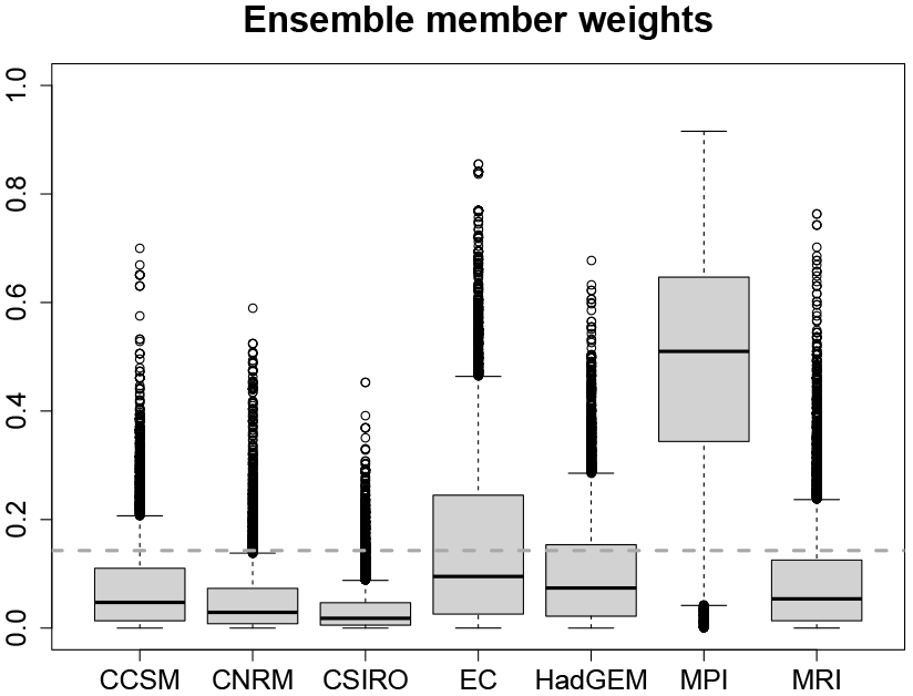
Figure 8Posterior ensemble member weights (λ) of the reconstruction. Prior weights (mean of λ) are denoted by the dashed line.
4.2.3 Added value of the reconstruction
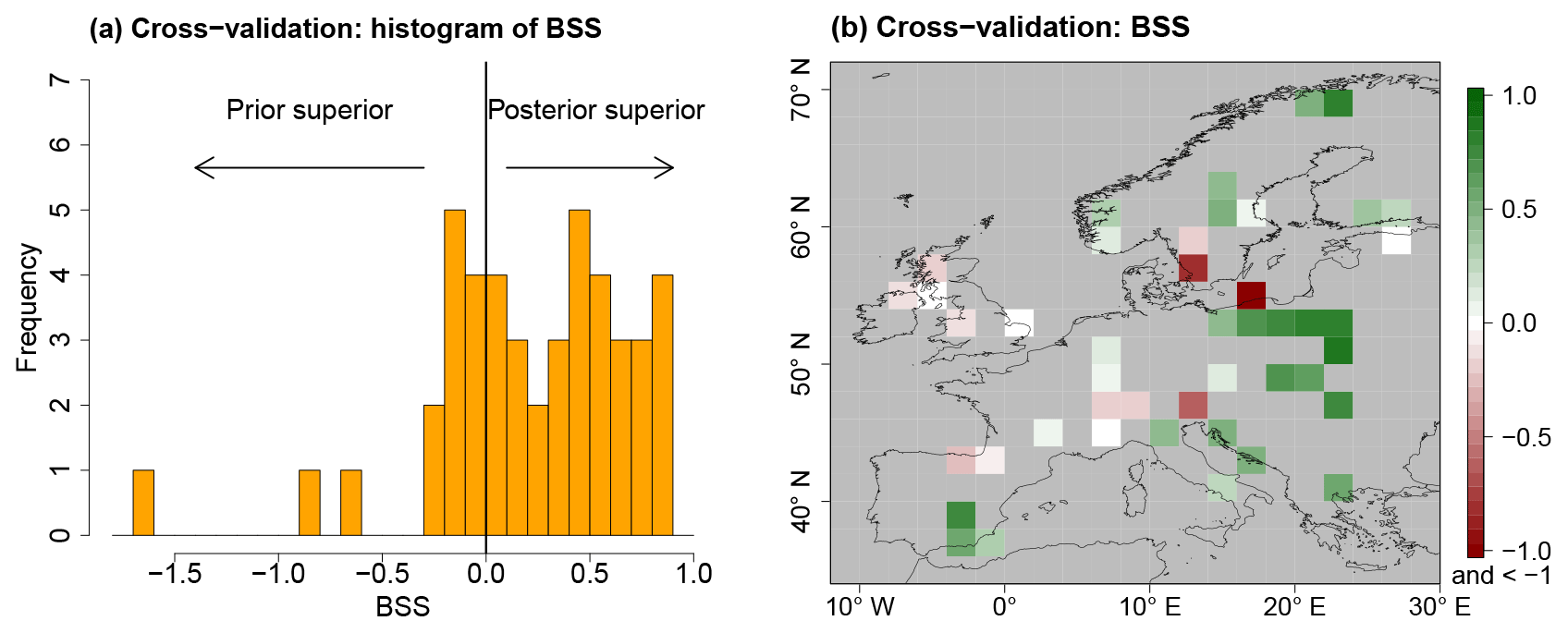
CVEs provide inside into the value that is added to the unconstrained PMIP3 ensemble, represented by process stage Eq. (7), by constraining it with the Simonis et al. (2012) synthesis. To quantify the added value, the BS from Eq. (20) is calculated for the unconstrained process stage, which is called BS(Prior), and compared to the BS of the posterior, BS(Posterior), calculated from leave-one-out CVEs. Then, the Brier skill score (BSS),
is computed, which is a measure of the added value of the spatial reconstruction. For positive BSS values, the posterior distribution is superior to the prior. On the other hand, the posterior distribution is inferior to the prior for negative values. This would indicate inconsistencies in the local proxy reconstructions or the existence of spurious correlations in the spatial covariance matrix.
For most left-out proxy samples, the BSS is positive (68.9 % of grid boxes) with a median of 0.28 (Fig. 9). The BSS values are predominantly positive for all regions but the British Islands and the Alps. This indicates high consistency of the reconstruction in large parts of the domain. In particular, consistent MTWA cooling in southern and eastern Europe in the local reconstructions compared to the prior distribution leads to cooling and a reduction of uncertainty in the posterior compared to the unconstrained PMIP3 ensemble. Similarly, the consistent MTWA and MTCO warming of the local reconstructions in the northeastern part of the domain leads to positive BSS values.
The persistent negative BSS values for the British Islands are evidence of a systematic issue. For this region, the uncertainty in the local reconstructions is larger than for other areas such that the local proxy records constrain the posterior less than the posterior ensemble member weights and some of the more distant proxy records. This leads to a reduction of the posterior uncertainty compared to the unconstrained PMIP3 ensemble but without improving the concordance of the mean state with the local reconstructions, which in turn results in negative BSS values. In and near the Alps, negative BSS might be a result of insufficient accounting for orographic effects in the different sources of information.
4.2.4 Joint versus separate MTWA and MTCO reconstructions
To study the effect of reconstructing MTWA and MTCO jointly compared to separately, additional reconstructions with only one climate variable are computed. Note that the interactions of MTWA and MTCO are twofold in the joint reconstruction: (a) the response functions have an interaction term, and (b) the process stage contains joint ensemble member weights for MTWA and MTCO as well as inter-variable correlations in the empirical correlation matrix.
The separate MTWA reconstruction is on average around 0.5 K warmer than the joint reconstruction, whereas the spatially averaged posterior mean of the separate MTCO reconstruction is 0.83 K cooler (Table 3). Hence, the seasonal difference is smaller in the joint reconstruction due to smoothing from the PMIP3 ensemble and slightly positive correlations between MTWA and MTCO in most of the joint local reconstructions. The MTWA-only reconstruction is warmer in most land areas, with the largest differences in southern and eastern Europe, but the differences are almost never significant on a 5 % level (Fig. 10a). As this part of the domain is best constrained by proxy data and the posterior ensemble member weights are similar to the joint reconstruction, it is likely that the additional warming is due to the missing interaction in the transfer function. On the other hand, the posterior ensemble member weights change a lot for the separate MTCO reconstruction, with HadGEM2-CC and MRI-CGCM3 being the models with the highest weights (mean λk of 0.426 and 0.199, respectively). Together with the less constrained transfer functions for MTCO than MTWA, this leads to a cooler reconstruction for most areas except some parts of the Mediterranean (Fig. 10b). The cooling is strongest in Scandinavia, the British Islands, the Norwegian Sea, and the Iberian Peninsula but almost never significant on a 5 % level. As these are the regions that are least constrained by proxy data, choosing different PMIP3 ensemble members affects the reconstruction more than in central Europe, where MTCO is best constrained by proxy data. The reconstruction uncertainties are of similar magnitude in the joint and the separate reconstructions (Table 3).
Table 3Summary measures for the joint MTWA and MTCO reconstructions (rows 1 and 2) and the separated reconstructions of MTWA (row 3) and MTCO (row 4). Numbers in brackets are minima and maxima of the corresponding 90 % CIs.
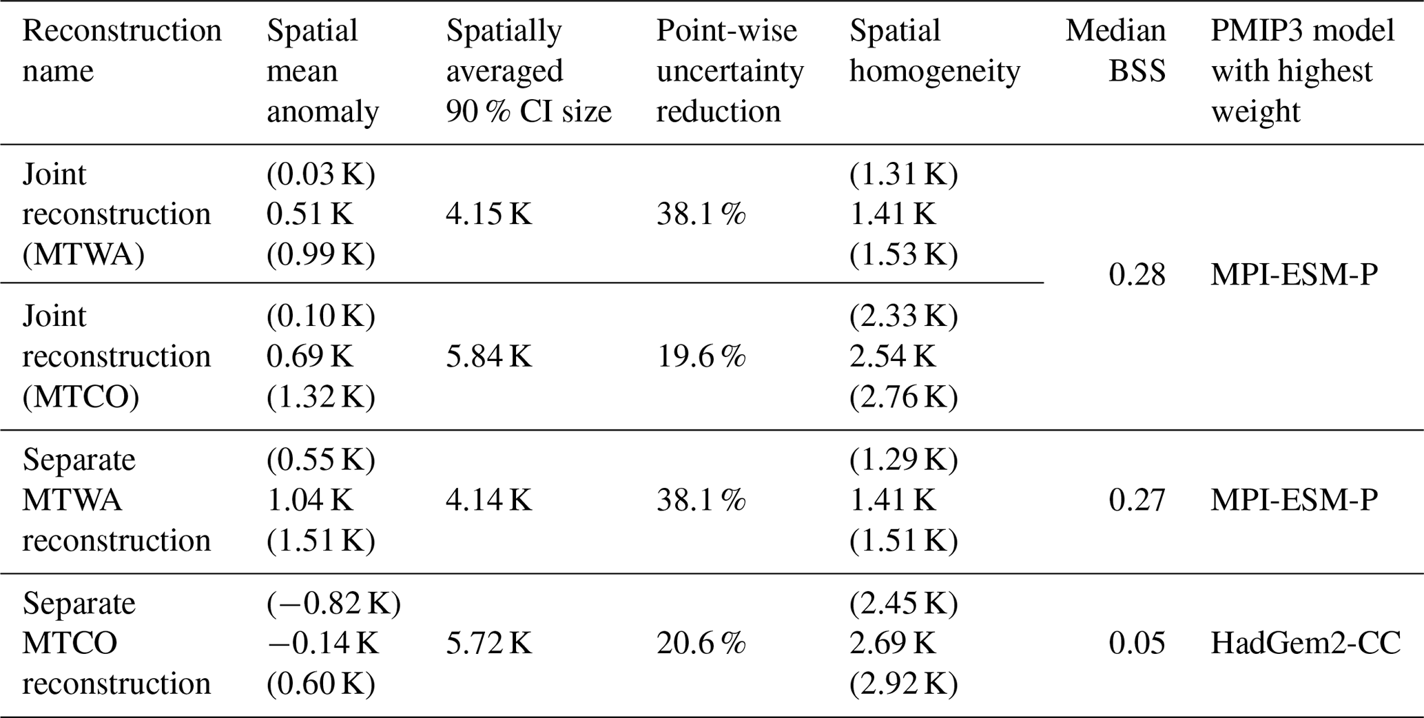
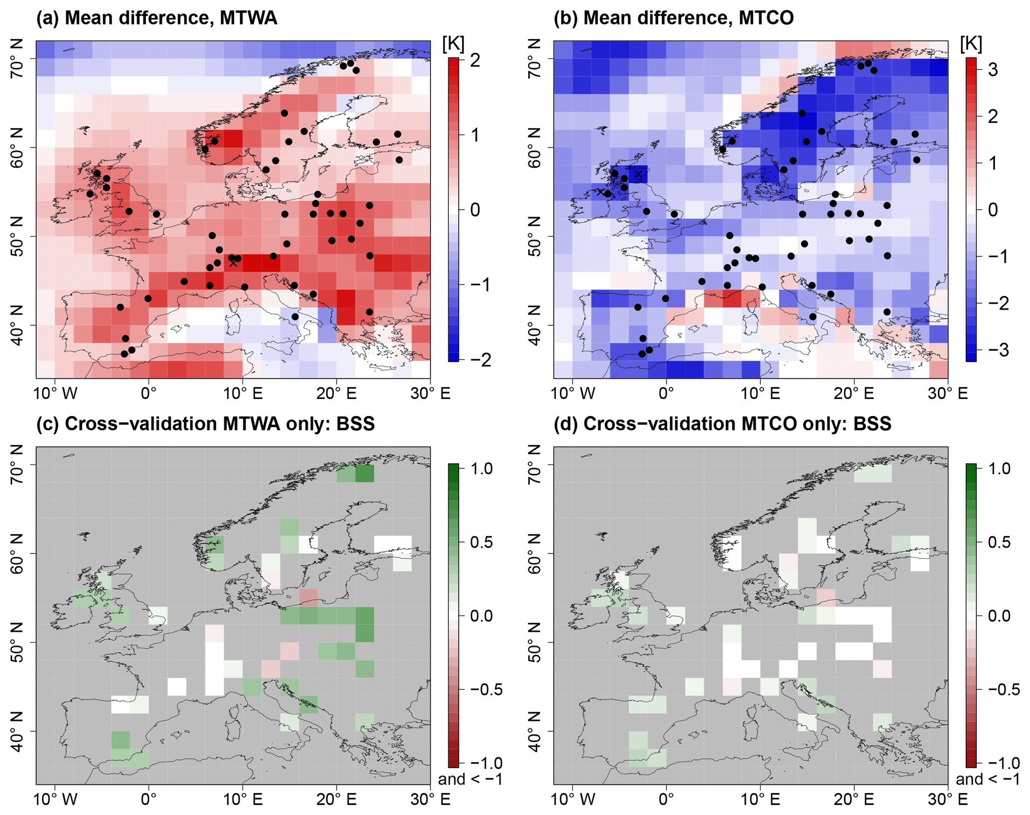
Figure 10Differences of joint and separate reconstructions of MTWA and MTCO. (a, b) Posterior mean difference; point-wise significant differences (5 % level) between the separate and the joint reconstructions are marked by black crosses. (c, d) BSS of the separate reconstructions. Black dots depict proxy samples.
The BSS pattern in the MTWA-only reconstruction is mostly the same as in the joint reconstruction except for slightly positive skill in the British Islands (Table 3, Fig. 10c). This shows that the added value of the joint reconstruction compared to the unconstrained PMIP3 ensemble is mainly determined by the MTWA reconstruction. On the other hand, the added value of the MTCO-only reconstruction is much smaller (Table 3, Fig. 10d) due to larger uncertainties in the local MTCO reconstructions.
The results show that the more constrained local MTWA reconstructions have a higher influence on the joint reconstruction than the local MTCO reconstructions. Reconstructing MTWA and MTCO jointly should in theory lead to a physically more reasonable reconstruction by creating samples drawn from the same combination of ensemble members. On the other hand, Rehfeld et al. (2016) show that multi-variable reconstructions from pollen assemblages can be biased when signals from a dominant variable are transferred to a minor variable. While the PITM model might be less sensitive to this issue than the weighted averaging transfer function used in Rehfeld et al. (2016) because it better respects the larger MTCO uncertainties, it will be the subject of future work to study whether joint or separate reconstructions lead to more reliable results.
5.1 Robustness of the reconstruction
Our approach is designed with the goal of being more suitable for sparse data situations than standard geostatistical models. To understand the robustness of the Bayesian framework with respect to the amount of data included in a proxy synthesis, five experiments with only half of the samples are performed, which are either selected to retain the spatial distribution of proxy samples or chosen randomly. In all of the tests, the general spatial structure of the posterior distribution, including the anomaly patterns, is preserved despite the fact that local anomalies and the magnitude of changes vary depending on the chosen proxy samples, which should be expected when such a large portion of the already sparse data is left out. Only the Norwegian Sea in the MTCO reconstruction changes substantially in some experiments. Plots from the experiments with reduced proxy samples are provided in the Supplement.
The mean spatial averages differ by up to 0.6 K for MTWA and MTCO, but none of the changes are significant on a 5 % level. In contrast, the uncertainty estimates are consistent across all five experiments with spatially averaged point-wise 90 % CIs that grow by up to 0.4 K from the reconstruction with the full proxy synthesis. In all experiments, the spatial homogeneity H is not significantly different from the values reported in Table 3, which shows that the spatial homogeneity is more controlled by the process stage than the proxy data. In all but one experiment, MPI-ESM-P remains the ensemble member with the largest weight λk, and the three ESMs that are favored neither in the MTWA nor in the MTCO reconstruction retain very low weights in all experiments. However, depending on whether proxy samples for which MTCO is much less constrained than MTWA are removed or not, the weights of the four models with the highest values in the joint and separate reconstructions can vary. This explains the MTCO changes in the Norwegian Sea as this is the region that is most influenced by the ensemble member weights. The experiments show that the reconstruction is robust with respect to the number of proxy samples as long as the remaining samples are informative and relatively uniformly distributed across space. In our example, this is not the case for the Norwegian Sea as no marine proxies are included.
The large PMIP3 ensemble spread for most grid boxes shows that the prior distribution, which is calculated from the ensemble, contains a wide range of possible states. In areas that are well constrained by proxy data, this large total uncertainty leads to a reconstruction that depends little on the climatologies of the ensemble members. Hence, in these areas, the reconstruction is not sensitive to the particular formulation of the process stage (compare with the Supplement). This shows that our method is applicable despite well-known model–data mismatches for the MH (Mauri et al., 2014). On the other hand, the spatial correlation structure controls the spread of local information into space. Different formulations of the spatial correlation matrix can lead to substantially different reconstructions in regions that are not well constrained by proxy samples and, in particular, a spatial covariance with too few spatial modes can lead to overly optimistic uncertainty estimates.
5.2 Comparison with previous reconstructions
Several reconstructions of European climate during the MH have been previously compiled. Here, we compare our reconstructions to those of Mauri et al. (2015), Simonis et al. (2012), and Bartlein et al. (2011).
Mauri et al. (2015) use a plant functional type modern analogue transfer function and a thin-plate spline interpolation for pollen samples stemming mostly from the European pollen database. Among other variables, summer and winter temperatures are reconstructed. We find a dipole anomaly structure similar to Mauri et al. (2015) in our reconstructions, with mostly positive anomalies in northern Europe and negative anomalies in southern Europe. In Mauri et al. (2015) and in our reconstruction, the Alps are the only region with significant warming in central and southern Europe for summer temperature. Generally, the amplitude of summer anomalies in the two reconstructions is similar, although locally there are differences, with cooler anomalies over southwestern Fennoscandia in our reconstruction and warmer anomalies in Finland. For winter temperatures, the cooling in the Mediterranean and the British Islands is less pronounced and spatially less consistent in our reconstruction than in Mauri et al. (2015). As for summer temperatures, we find smaller anomalies in southern Fennoscandia. In contrast, our reconstruction shows higher anomalies in northern Scandinavia.
The same pollen dataset and another version of PITM are used in Simonis et al. (2012) to reconstruct July and January temperature such that differences between the two reconstructions are mostly related to the different smoothing technique. Simonis et al. (2012) minimize a cost function that combines pollen samples with an advection–diffusion model that is driven by insolation changes between the MH and today. In Simonis et al. (2012), the dipole structure is not found in the same way as in our reconstruction. Both reconstructions share positive summer temperature anomalies in northern Europe as well as negative anomalies in central Europe and the Iberian Peninsula. Unlike our reconstruction, Simonis et al. (2012) find positive anomalies in southeastern Europe. For winter temperatures, the reconstruction of Simonis et al. (2012) shows an east–west dipole in contrast to the northeast to southwest dipole in our reconstruction. This different structure might be due to the smaller proxy data control of the winter reconstructions, which leads to a higher importance of the interpolation schemes.
A reconstruction designed to evaluate the PMIP3 simulations was provided by Bartlein et al. (2011). They combine a large number of pollen-based local reconstructions from the literature to produce a gridded product of six climate variables including MTWA and MTCO. In contrast to our reconstruction, the local reconstructions used are not smoothed across space but only within a grid box. Their results show a dipole structure but less pronounced than in our reconstruction. In particular, they find a cooling for eastern Fennoscandia in summer, a much smaller warming of northern Fennoscandia, and a warming in Germany and France. On the other hand, the reported anomalies in Bartlein et al. (2011) for the Mediterranean and eastern Europe are similar to our results.
The comparisons show that patterns like the dipole-type anomaly structure, which are not present in the PMIP3 ensemble, seem to be consistent across reconstructions with pollen transfer functions. While some of the differences between the existing literature and our results can be explained by the used transfer functions and proxy syntheses, the choice of an appropriate interpolation method plays an important role, too, especially in areas with very sparse and weakly informative proxy data.
5.3 Climate model inadequacy and process stage structure
To account for inadequacies of climate models in simulating past climate states, we introduced flexible ensemble member weights λ and the shrinkage matrix approach that combines the empirical covariance matrix of the climate ensemble with an independent correlation matrix. Combining ensemble filtering methods with additional techniques to correct model biases in a physically consistent way is an important but also challenging direction of future work on climate field reconstructions, as a balance has to be found between under-dispersion of the posterior distribution by inducing physical structures and over-fitting to noisy proxy data by enhancing the degrees of freedom. Beyond the strategies implemented in this work, some directions that can be envisaged are an increase in permitted spatial structures in the prior mean by adding patterns calculated from alternative physically motivated models and the introduction of multiple shrinkage targets in the spatial covariance matrix (Gray et al., 2018).
The strong effect of the covariance regularization technique on the reconstructions might originate from the small ensemble size. This hypothesis can be tested when more simulations with sufficient resolution become available, for example from the PMIP4 project. In addition, it indicates that the modes of the empirical covariance matrix do not optimally explain the spatial variability of the climate and the corresponding uncertainty structures. The difference between under-dispersive behavior in ITEs with glasso models and over-dispersion for shrinkage models suggests that the optimal number of effective degrees of freedom lies between those two models. However, an optimization procedure for the number of spatial modes in the covariance matrix is not straightforward and left for future research.
In the current study, we use a fixed prior distribution for the ensemble member weights (compare with Sect. 3.3). An extension of this model would be to let the proxy data inform whether more balanced weights should be favored or weights with one dominant ensemble member. This can be achieved by using a hyperprior that controls the concentration of the weights.
We presented a new method for probabilistic spatial reconstructions of paleoclimate. The approach combines the strengths of pollen and macrofossil records, which provide information about the local climate state, and climate simulations, which downscale forcing conditions to physically consistent regional climate patterns. Thus, we reconstruct physically reasonable spatial fields, which are consistent with a given proxy synthesis. Our framework can deal with probabilistic transfer functions, which are nonlinear and non-Gaussian, such that an extension to a wide range of proxies and associated transfer functions is possible.
Using ITEs and CVEs, we showed that robust spatial reconstructions with Bayesian filtering methods that exhibit small biases and are not under-dispersed are possible as long as the statistical framework is flexible enough to account for deficiencies of climate simulations and to avoid filter degeneracy, which can emerge due to small ensemble sizes and biases in climate simulations. The resulting model, which is used for spatial reconstructions of European MH climate, uses a weighted average of the involved ensemble member climatologies and a shrinkage matrix approach for spatial interpolation and structural extrapolation of the proxy data.
We apply our framework to reconstruct MTWA and MTCO in Europe during the MH using the proxy synthesis of Simonis et al. (2012) and the PMIP3 MH ensemble. Brier scores from cross-validations reveal that the spatial reconstruction predominantly adds value to the unconstrained PMIP3 ensemble, and analyses of the spatial homogeneity of the posterior distribution indicate a reasonable degree of spatial smoothing. The large-scale spatial patterns of our reconstruction are in agreement with previous work (Mauri et al., 2015; Bartlein et al., 2011). As the posterior mean is more similar to the local proxy reconstructions than to the prior mean for most terrestrial areas, we see that a reconstruction, which is in line with reconstructions that do not include simulation output, is possible despite well-known model–data mismatches (Mauri et al., 2014). Our framework provides a way to quantitatively test hypotheses in paleoclimatology and to assess the consistency of a given proxy synthesis.
R code for computing reconstructions with the presented Bayesian framework is provided in a Bitbucket repository available under https://bitbucket.org/nils_weitzel/spatial_reconstr_repo (Weitzel, 2019). The pollen and macrofossil synthesis is published in Simonis (2009). It is available in the Bitbucket repository. The PMIP3 MH simulations are available in the CMIP5 archives. In this study, they were downloaded from the DKRZ long-term archive CERA (https://cera-www.dkrz.de, last access: 27 April 2016). The modern climate data were downloaded from the University of East Anglia Climatic Research Unit, available at http://www.cru.uea.ac.uk/data/ (Harris et al., 2017). The vegetation data for transfer function calibration were provided by Thomas Litt and Norbert Kühl.
To determine the glasso penalty parameter ξ, we first recognize that for values smaller than ξ=0.3 the resulting matrices become numerically unstable in our application due to the small ensemble size. Five values for ξ were tested: 0.3, 0.5, 0.7, 1.0, and 2.0. Larger values lead to sparser precision matrices and therefore to weaker spatial correlations. For each of the five parameters, we perform CVEs with the RM and compare the resulting BS (see Sect. 4.1.2). While the smallest penalty parameters have the best mean BS, the differences are generally small (see the Supplement). However, the influence of the penalty term in Eq. (14) on the overall regression increases from 79.5 % for ξ=0.3 to 98.5 % for ξ=2.0. Based on these diagnostics, we choose ξ=0.3 for the reconstructions in this study. The sensitivity of the reconstruction with respect to ξ is further studied in the Supplement.
The shrinkage target Φ is defined on a regular lat–long grid following the stochastic partial differential equation approach of Lindgren et al. (2011). This approach allows for a computationally efficient approximation of Matérn covariances with parameters that are physically motivated in the context of stochastic Laplace equations, which model diffusive transport of a stochastic forcing. Setting , the range parameter ρ is rewritten as a scale parameter ζ2. Moreover, we let the anisotropy parameter ν parameterize a diagonal diffusion matrix . Then, the stochastic partial differential equation from which Φ is deduced is given by
𝒲 denotes white noise, and X is the stationary Gaussian random field that solves Eq. (B1). Discretizing this equation with linear finite elements and using a diagonal approximation of the involved mass matrix leads to a GMRF with correlation matrix (Lindgren et al., 2011). We use degrees as a distance unit on the regular lat–long grid instead of meters, which means that the decorrelation length depends on the latitude. This better reflects the mostly shorter decorrelation lengths at higher latitudes. Φ is constructed from by combining spatial correlation matrices of type for each climate variable in a block diagonal structure. Different parameters ρ and ν are fitted for each climate variable.
The Metropolis-within-Gibbs approach samples (asymptotically) from the full conditional distributions of each variable, i.e., the distribution of the variable given all other variables. Some variables are treated block-wise. In this Appendix, we detail the conditional distributions that are used for sampling.
To sample the transfer function parameters, we introduce augmented variables as described in Sect. 3.4. Their full conditional distribution is given by
Including the Gaussian prior defined in Sect. 3.2, the full conditional of βT is Gaussian distributed:
Here, X is a matrix with rows XC(l) for l=1, …, L(T), Γ is a diagonal matrix with entries , B is the 6×6 prior covariance matrix of βT, and κT is a vector with entries , where PT(l) is the presence or absence of taxa T in observation l. In our case, B is a diagonal matrix with all values equal to 10. Details on the definition of PG variables and the augmented Gibbs sampler can be found in Polson et al. (2013).
Sampling from ϑ depends on the specific version of the process stage used. In the RM, is influenced by its prior and by the Gaussian distribution of Cp given λ:
This full conditional does not follow a probability distribution from which we can sample directly. Therefore, a random-walk-type Metropolis–Hastings update is used for updating λ.
In the KM, the full conditional of is Dirichlet distributed given and its Dirichlet prior:
Given ω and Cp, z is categorically distributed:
If shrinkage covariance matrices are used, the parameters (α,ρ,ν) have to be chosen in each MCMC step from one of the K=7 predefined parameter sets. We use a uniform prior. Then, the full conditional of τ that indexes the parameter sets is given by
where is given according to conditioning on the process stage parameters of the GM, RM, or KM. We update τ using a Metropolis–Hastings step with independent proposals, which choose τ=k with probability .
We update Cp(x) for x∈xP sequentially using random walk Metropolis–Hastings sampling. The set of all grid boxes besides x is denoted by Yx, and let be the block of the inverse covariance matrix containing the rows a and columns b. Then, the full conditional distribution of Cp(x) depends on the pollen samples Pp(s) with location xs=x, the climate Cp(Yx) at the other locations, and process stage parameters ϑ. It does not follow a standard distribution:
Conditioned on Cp(xP) and ϑ, Cp(xQ) follows a Gaussian distribution:
As described in Sect. 3.4, the multi-modality of the KM in combination with the high dimensionality of the posterior makes the standard MCMC algorithm very inefficient. In our specific formulation the inefficiency is manifested in a very slow mixing of z because, conditioned on Cp, the likelihood of choosing a new model zk from one MCMC step to the next one is very small. This problem could be shifted to other variables by integrating out z, but then the conditional Gaussian structure of Cp would be lost, which would lead to new challenges for generating efficient MCMC strategies. Therefore, we apply an MC3 or parallel tempering strategy (Geyer, 1991; Altekar et al., 2004; Werner and Tingley, 2015).
We run A MCMC chains in parallel, and after every M steps, we use an additional Metropolis–Hastings step to swap the states of the Markov chains a1 and a2 with probability , where is calculated from the Metropolis–Hastings odds ratio. The Markov chains are created by exponentiating the process stage and the data stage by constants . The first Markov chain (ν1=1) asymptotically retains the original posterior distribution for all variables, whereas the subsequent chains sample from a flatter posterior distribution, in which it is easier to jump from one kernel to another. Following empirical testing, we run the European reconstructions with A=8 parallel chains, levels ν1=1, , …, , and swaps after every M=30 steps. The pseudo-code for the MC3 algorithm is given in the Supplement.
The supplement related to this article is available online at: https://doi.org/10.5194/cp-15-1275-2019-supplement.
NW performed the theoretical work, the model and graphics implementation, and wrote the major part of the text. AH and CO proposed the reconstruction framework, contributed to the discussion of results, and commented on the different versions of the paper.
The authors declare that they have no conflict of interest.
This article is part of the special issue “Paleoclimate data synthesis and analysis of associated uncertainty (BG/CP/ESSD inter-journal SI)”. It is not associated with a conference.
Nils Weitzel was additionally supported by the German Research Foundation (code RE3994-2/1) and the National Center for Atmospheric Research (NCAR). NCAR is funded by the National Science Foundation. We acknowledge all groups involved in producing and making available the PMIP3 multi-model ensemble. We acknowledge the World Climate Research Programme's Working Group on Coupled Modelling, which is responsible for CMIP5. For CMIP5 the US Department of Energy’s Program for Climate Model Diagnosis and Intercomparison provides coordinating support and led the development of software infrastructure in partnership with the Global Organization for Earth System Science Portals. We thank Douglas Nychka for helpful ideas to speed up the MCMC algorithm. We thank two anonymous referees and the editor for their interesting and helpful comments, which facilitated a substantial improvement of this paper.
This research has been supported by the German Federal Ministry of Education and Research (BMBF) as a Research for Sustainability initiative (FONA; https://www.fona.de, last access: 30 May 2019) through the Palmod project (grant no. FKZ: 01LP1509D).
This paper was edited by André Paul and reviewed by two anonymous referees.
Altekar, G., Dwarkadas, S., Huelsenbeck, J. P., and Ronquist, F.: Parallel Metropolis coupled Markov chain Monte Carlo for Bayesian phylogenetic inference, Bioinformatics, 20, 407–415, 2004. a
Anderson, J. L. and Anderson, S. L.: A Monte Carlo Implementation of the Nonlinear Filtering Problem to Produce Ensemble Assimilations and Forecasts, Mon. Weather Rev., 127, 2741–2758, 1999. a
Annan, J. D. and Hargreaves, J. C.: A new global reconstruction of temperature changes at the Last Glacial Maximum, Clim. Past, 9, 367–376, https://doi.org/10.5194/cp-9-367-2013, 2013. a
Bartlein, P., Harrison, S., Brewer, S., Connor, S., Davis, B., Gajewski, K., Guiot, J., Harrison-Prentice, T., Henderson, A., Peyron, O., Prentice, I., Scholze, M., Seppä, H., Shuman, B., Sugita, S., Thompson, R., Viau, A., Williams, J., and Wu, H.: Pollen-based continental climate reconstructions at 6 and 21 ka: a global synthesis, Clim. Dynam., 37, 775–802, 2011. a, b, c, d, e
Birks, H. J. B., Heiri, O., Seppä, H., and Bjune, A. E.: Strengths and Weaknesses of Quantitative Climate Reconstructions Based on Late-Quaternary Biological Proxies, The Open Ecology Journal, 3, 68–110, 2010. a
Braconnot, P., Harrison, S. P., Otto-Bliesner, B., Abe-Ouchi, A., Jungclaus, J., and Peterschmitt, J.-Y.: The Paleoclimate Modeling Intercomparison Project contribution to CMIP5, CLIVAR Exchanges, 56, 15–19, 2011. a, b
Bradley, R. S.: Paleoclimatology – Reconstructing Climates of the Quaternary, Academic Press, Oxford, 3 Edn., 324–327, 2015. a, b
Brier, G.: Verification of Forecasts Expressed in Terms of Probability, Mon. Weather Rev., 78, 1–3, 1950. a
Brooks, S. P. and Gelman, A.: General Methods for Monitoring Convergence of Iterative Simulations, J. Comput. Graph. Stat., 7, 434–455, 1998. a
Carrassi, A., Bocquet, M., Bertino, L., and Evensen, G.: Data assimilation in the geosciences. An overview on methods, issues and perspectives, WIREs Climate Change, available at: https://arxiv.org/abs/1709.02798 (last acces: 30 May 2019), 2018. a, b
Dee, S., Steiger, N. J., Hakim, G. J., and Emile-Geay, J.: On the utility of proxy system models for estimating climate states over the common era, J. Adv. Model. Earth Sy., 8, 1164–1179, 2016. a
Friedman, J., Hastie, T., and Tibshirani, R.: Sparse inverse covariance estimation with the graphical lasso, Biostatistics, 9, 432–441, 2008. a
Gebhardt, C., Kühl, N., Hense, A., and Litt, T.: Multi-Scale Processes and the Reconstruction of Palaeoclimate, in: Dynamics of Multiscale Earth Systems, edited by: Neugebauer, H. J. and Simmer, C., Springer, Berlin, 325–336, 2003. a
Gebhardt, C., Kühl, N., Hense, A., and Litt, T.: Reconstruction of Quaternary temperature fields by dynamically consistens smoothing, Clim. Dynam., 30, 421–437, 2008. a, b, c, d, e, f
Gelman, A., Carlin, J., Stern, H., Dunson, D., Vehtari, A., and Rubin, D.: Bayesian data analysis, vol. 3, Chapman & Hall, CRC Press, Boca Raton, 2013. a, b
Geyer, C.: Markov chain Monte Carlo maximum likelihood, in: Computing Science and Statistics: Proceedings of the 23rd Symposium on the Interface, Interface Foundation, edited by: Keramidas, E. M., Fairfax Station, 156–163, 1991. a, b
Gneiting, T. and Raftery, A. E.: Strictly Proper Scoring Rules, Prediction, and Estimation, J. Am. Stat. Assoc., 102, 359–378, 2007. a
Gomez-Navarro, J. J., Werner, J., Wagner, S., Luterbacher, J., and Zorita, E.: Establishing the skill of climate field reconstruction techniques for precipitation with pseudoproxy experiments, Clim. Dynam., 45, 1395–1413, 2015. a
Gray, H., Leday, G. G., Vallejos, C. A., and Richardson, S.: Shrinkage estimation of large covariance matrices using multiple shrinkage targets, arXiv:1809.08024v1, 1–32, available at: https://arxiv.org/abs/1809.08024v1 (last access: 30 May 2019), 2018. a
Hannart, A. and Naveau, P.: Estimating high dimensional covariance matrices: A new look at the Gaussian conjugate framework, J. Multivariate Anal., 131, 149–162, 2014. a
Harris, I. and Jones, P.: CRU TS4.01: Climatic Research Unit (CRU) Time-Series (TS) version 4.01 of high-resolution gridded data of month-by-month variation in climate (January 1901–December 2016), https://doi.org/10.5285/58a8802721c94c66ae45c3baa4d814d0 (last access: 30 May 2019), 2017. a
Harris, I., Jones, P., Osborn, T., and Lister, D.: Updated high-resolution grids of monthly climatic observations – the CRU TS3.10 Dataset, Int. J. Climatol., 34, 623–642, 2014. a
Haslett, J., Whiley, M., Bhattacharya, S., Salter-Townshend, M., Wilson, S. P., Allen, J., Huntley, B., and Mitchell, F.: Bayesian paleoclimate reconstruction, J. R. Stat. Soc. A Stat., 169, 395–438, 2006. a
Hegerl, G. and Zwiers, F.: Use of models in detection and attribution of climate change, WIREs Clim Change, 2, 570–591, 2011. a
Holden, P. B., Birks, H. J. B., Brooks, S. J., Bush, M. B., Hwang, G. M., Matthews-Bird, F., Valencia, B. G., and van Woesik, R.: BUMPER v1.0: a Bayesian user-friendly model for palaeo-environmental reconstruction, Geosci. Model Dev., 10, 483–498, https://doi.org/10.5194/gmd-10-483-2017, 2017. a
Holmström, L., Ilvonen, L., Seppä, H., and Veski, S.: A Bayesian Spatiotemporal Model for Reconstructing Climate from Multiple Pollen Records, Ann. Appl. Stat., 9, 1194–1225, 2015. a
Iversen, J.: Viscum, Hedera and Ilex as climate indicators, Geologiska Foereningens i Stockholm foerhandlingar, 66, 463–483, 1944. a
Jones, P., New, M., Parker, D., Martin, S., and Rigor, I.: Surface air temperature and its variations over the last 150 years, Rev. Geophys., 37, 173–199, 1999. a
Knutti, R., Furrer, R., Tebaldi, C., Cermak, J., and Meehl, G. A.: Challenges in combining projections from multiple climate models, J. Clim., 23, 2739–2758, 2010. a
Krishnamurti, T. N., Kishtawal, C. M., LaRow, T. E., Bachiochi, D. R., Zhang, Z., Williford, C. E., Gadgil, S., and Surendran, S.: Improved Weather and Seasonal Climate Forecasts from Multimodel Superensemble, Science, 285, 1548–1550, 1999. a
Kühl, N., Gebhardt, C., Litt, T., and Hense, A.: Probability Density Functions as Botanical-Climatological Transfer Functions for Climate Reconstruction, Quarternary Res., 58, 381–392, 2002. a, b, c, d
Kühl, N., Litt, T., Schölzel, C., and Hense, A.: Eemian and Early Weichselian temperature and precipitation variability in northern Germany, Quarternary Sci. Rev., 26, 3311–3317, 2007. a
Li, B., Nychka, D. W., and Ammann, C. M.: The Value of Multiproxy Reconstruction of Past Climate, J. Am. Stat. Assoc., 105, 883–895, 2010. a
Lindgren, F., Rue, H., and Lindström, J.: An explicit link between Gaussian fields and Gaussian Markov random fields: the stochastic partial differential equation approach, J. R. Stat. Soc. B Met., 73, 423–498, 2011. a, b, c
Liu, B., Ait-El-Fquih, B., and Hoteit, I.: Efficient Kernel-Based Ensemble Gaussian Mixture Filtering, Mon. Weather Rev., 144, 781–800, 2016. a
Liu, F., Bayarri, M., and Berger, J.: Modularization in Bayesian analysis, with emphasis on analysis of computer models, Bayesian Anal., 4, 119–150, 2009. a
MacKenzie, D. I., Nichols, J. D., Lachman, G. B., Droege, S., Royle, J. A., and Langtimm, C. A.: Estimating site occupancy rates when detection probabilities are less than one, Ecology, 83, 2248–2255, 2002. a
Matheson, J. and Winkler, R.: Scoring Rules for Continuous Probability Distributions, Manage. Sci., 22, 1087–1096, 1976. a
Mauri, A., Davis, B. A. S., Collins, P. M., and Kaplan, J. O.: The influence of atmospheric circulation on the mid-Holocene climate of Europe: a data–model comparison, Clim. Past, 10, 1925–1938, https://doi.org/10.5194/cp-10-1925-2014, 2014. a, b
Mauri, A., Davis, B., Collins, P., and Kaplan, J.: The climate of Europe during the Holocene: a gridded pollen-based reconstruction and its multi-proxy evaluation, Quaternary Sci. Rev., 112, 109–127, 2015. a, b, c, d, e, f
Ohlwein, C. and Wahl, E. R.: Review of probabilistic pollen-climate transfer methods, Quaternary Sci. Rev., 31, 17–29, 2012. a
Parnell, A. C., Sweeney, J., Doan, T. K., Salter-Townshend, M., Allen, J. R., Huntley, B., and Haslett, J.: Bayesian inference for palaeoclimate with time uncertainty and stochastic volatility, J. Roy. Stat. Soc. C-Appl., 64, 115–138, 2015. a, b, c
Parnell, A. C., Haslett, J., Sweeney, J., Doan, T. K., Allen, J. R., and Huntley, B.: Joint Palaeoclimate reconstruction from pollen data via forward models and climate histories, Quarternary Sci. Rev., 151, 111–126, 2016. a
Plummer, M., Best, N., Cowles, K., and Vines, K.: CODA: Convergence Diagnosis and Output Analysis for MCMC, R News, 6, 7–11, 2006. a
Polson, N. G., Scott, J. G., and Windle, J.: Bayesian Inference for Logistic Models Using Pólya–Gamma Latent Variables, J. Am. Stat. Assoc., 108, 1339–1349, 2013. a, b, c
Rehfeld, K., Trachsel, M., Telford, R. J., and Laepple, T.: Assessing performance and seasonal bias of pollen-based climate reconstructions in a perfect model world, Clim. Past, 12, 2255–2270, https://doi.org/10.5194/cp-12-2255-2016, 2016. a, b
Rue, H. and Held, L.: Gaussian Markov random fields : theory and applications, Chapman & Hall/CRC (Taylor & Francis Group), Boca Raton, 2005. a
Schölzel, C., Hense, A., Hübl, P., Kühl, N., and Litt, T.: Digitization and geo-referencing of botanical distribution maps, J. Biogeogr., 29, 851–856, 2002. a, b
Silverman, B.: Density Estimation for Statistics and Data Analysis, vol. 26 of Monographs on Statistics and Applied Probability, Chapman & Hall/CRC, Boca Raton, 1986. a, b, c
Simonis, D.: Reconstruction of possible realizations of the Late Glacial and Holocene near surface climate in Central Europe, Dissertation, Meteorologisches Institut der Rheinischen Friedrich-Wilhelms-Universität Bonn, 2009. a, b, c, d, e, f
Simonis, D., Hense, A., and Litt, T.: Reconstruction of late Glacial and Early Holocene near surface temperature anomalies in Europe and their statistical interpretation, Quaternary Int., 274, 233–250, 2012. a, b, c, d, e, f, g, h, i, j, k, l, m, n, o, p
Steiger, N. J., Hakim, G. J., Steig, E. J., Battisti, D. S., and Roe, G. H.: Assimilation of Time-Averaged Pseudoproxies for Climate Reconstruction, J. Clim., 27, 426–441, 2014. a
Stolzenberger, S.: Untersuchungen zu botanischen Paläoklimatransferfunktionen, Diploma thesis, Meteorologisches Institut der Rheinischen Friedrich-Wilhelms-Universität Bonn, 2011. a, b
Stolzenberger, S.: On the probabilistic evaluation of decadal and paleoclimate model predictions, Dissertation, Meteorologisches Institut der Rheinischen Friedrich-Wilhelms-Universität Bonn, 2017. a, b
Tawn, N. G. and Roberts, G. O.: Accelerating Parallel Tempering: Quantile Tempering Algorithm (QuanTA), Adv. Appl. Probab., in press, available at: https://arxiv.org/abs/1808.10415v1 (Last access: 30 May 2019), 2019. a
Thuiller, W.: BIOMOD – optimizing predictions of species distributions and projecting potential future shifts under global change, Glob. Change Biol., 9, 1353–1362, 2003. a
Tingley, M. P. and Huybers, P.: A Bayesian Algorithm for Reconstructing Climate Anomalies in Space and Time. Part I: Development and Applications to Paleoclimate Reconstruction Problems, J. Clim., 23, 2759–2781, 2010. a, b
Tingley, M. P., Craigmile, P. F., Haran, M., Li, B., Mannshardt, E., and Rajaratnam, B.: Piecing together the past: statistical insights into paleoclimatic reconstructions, Quaternary Sci. Rev., 35, 1–22, 2012. a
Weitzel, N: Spatial_reconstr_repo, available at: https://bitbucket.org/nils_weitzel/spatial_reconstr_repo, last access: 30 May 2019.
Werner, J. P. and Tingley, M. P.: Technical Note: Probabilistically constraining proxy age–depth models within a Bayesian hierarchical reconstruction model, Clim. Past, 11, 533–545, https://doi.org/10.5194/cp-11-533-2015, 2015. a
Windle, J., Polson, N. G., and Scott, J. G.: BayesLogit: Bayesian logistic regression, available at: http://cran.r-project.org/web/packages/BayesLogit/index.html (last access: 30 May 2019), 2013. a
Windle, J., Polson, N. G., and Scott, J. G.: Sampling Pólya-Gamma random variates: alternate and approximate techniques, arXiv:1405.0506v1, available at: https://arxiv.org/abs/1405.0506v1 (last access: 30 May 2019), 2014. a
Yang, Z. and Zhu, T.: The good, the bad, and the ugly: Bayesian model selection produces spurious posterior probabilities for phylogenetic trees, arXiv:1810.05398v1, available at: https://arxiv.org/abs/1810.05398v1 (last access: 30 May 2019), 2018. a
- Abstract
- Introduction
- Data
- Methods
- Results
- Discussion and possible extensions
- Conclusions
- Code and data availability
- Appendix A: Determination of glasso penalty parameter
- Appendix B: Shrinkage target matrix
- Appendix C: Full conditional distributions
- Appendix D: Metropolis coupled Markov chain Monte Carlo algorithm
- Author contributions
- Competing interests
- Special issue statement
- Acknowledgements
- Financial support
- Review statement
- References
- Supplement