the Creative Commons Attribution 4.0 License.
the Creative Commons Attribution 4.0 License.
 | 02 Aug 2019
Impact of different estimations of the background-error covariance matrix on climate reconstructions based on data assimilation
Veronika Valler
Jörg Franke
Stefan Brönnimann
Data assimilation has been adapted in paleoclimatology to reconstruct past climate states. A key component of some assimilation systems is the background-error covariance matrix, which controls how the information from observations spreads into the model space. In ensemble-based approaches, the background-error covariance matrix can be estimated from the ensemble. Due to the usually limited ensemble size, the background-error covariance matrix is subject to the so-called sampling error. We test different methods to reduce the effect of sampling error in a published paleoclimate data assimilation setup. For this purpose, we conduct a set of experiments, where we assimilate early instrumental data and proxy records stored in trees, to investigate the effect of (1) the applied localization function and localization length scale; (2) multiplicative and additive inflation techniques; (3) temporal localization of monthly data, which applies if several time steps are estimated together in the same assimilation window. We find that the estimation of the background-error covariance matrix can be improved by additive inflation where the background-error covariance matrix is not only calculated from the sample covariance but blended with a climatological covariance matrix. Implementing a temporal localization for monthly resolved data also led to a better reconstruction.


Estimating the state of the atmosphere in the past is important to enhance our understanding of the natural climate variability, the underlying mechanisms of past climate changes and their impacts. To infer past climate states, two basic sources of information are available: observations and numerical models. Climate models constrained with realistic, time-dependent external forcings provide fields that are consistent with these forcings and the model physics. Observations can be instrumental meteorological measurements, which are mainly available from the mid-19th century. Prior to this time, information from proxies stored in natural archives (like trees, speleothems, marine sediments, ice cores) or documentary data can be exploited. Observations provide important local information; however, their spatial and temporal coverage is sparse.
In recent years, a novel technique, the data assimilation (DA) approach, has been adapted for paleoclimatological research. DA creates a framework to combine information from different sources. If information from observations is optimally blended with climate model simulations, the result is the best estimate of the climatic state, given the observations, given the external forcings and given the known climate physics. The field of paleoclimate data assimilation (PDA) has undergone profound developments, and many DA techniques have been implemented to reconstruct past climate states, such as forcing singular vectors and pattern nudging (Widmann et al., 2010), selection of ensemble members (Goosse et al., 2006; Matsikaris et al., 2015), particle filters (e.g., Goosse et al., 2010), the variation approach (Gebhardt et al., 2008), the Kalman filter and its modifications (e.g., Bhend et al., 2012; Hakim et al., 2016; Franke et al., 2017a; Steiger et al., 2018). However, there are still unresolved problems and thus a need for improvements of how to best combine observations with climate model simulations.
One popular DA method is the Kalman filter (KF; Kalman, 1960). In standard applications, the processes of the KF can be summarized in two main steps (Ide et al., 1997). In the update step, the background state and the uncertainty of the background state provided by the model simulation are adjusted by assimilating new observations. In the forecast step, the updated state, called the analysis, and the uncertainty of the analysis are propagated forward in time. These processes are repeated when new observations become available. However, in PDA, the forecast step is usually neglected; that is, the filter is used offline (e.g., Franke et al., 2017a). Because the process is not cycled, the background state is obtained from a precomputed model simulation. In some previous PDA studies, the background state is constructed once from the model simulation, and later, the same state is used in every assimilation window (Steiger et al., 2018, and references therein); we refer to them as stationary (forcing-independent) offline DA methods. In other PDA studies, the background state is specific for the current assimilation window; that is, the state changes in each assimilation window according to the forcings (Bhend et al., 2012; Franke et al., 2017a); we call them transient (forcing-dependent) offline DA methods.
An essential component of the KF is the uncertainty of the background state. In ensemble-based approaches, an ensemble of the background state provides estimation of the truth, represented by the ensemble mean, and the perturbations from the mean are used to estimate the uncertainty, represented by the background-error covariance matrix. Ensemble-based KFs are approximations of the KF, because the true state is usually sampled with a few tens to a few hundreds of ensemble members. The limited ensemble size leads to errors in the estimation of the background-error covariance matrix. This effect is known as the sampling error.
Two methods are commonly used in online ensemble-based KF approaches to reduce the negative effect of sampling error: inflation (e.g., Anderson and Anderson, 1999) and localization (e.g., Hamill et al., 2001) of the background-error covariance matrix. A simple inflation technique is the multiplicative inflation (Anderson and Anderson, 1999), which compensates for potential underestimation of the analysis error. Multiplicative inflation helps to maintain a more realistic distribution of the ensemble members by increasing the deviation of the members from the ensemble mean at each DA cycle (Anderson and Anderson, 1999). However, the underestimation of the analysis error is of minor importance in offline approaches, because the ensemble members are not propagated forward in time. Covariance inflation, besides reducing the sampling error, can also account for underestimated model error. In the additive inflation technique, the covariances are inflated by, e.g., adding an additional error term to the background-error covariances (Houtekamer et al., 2005). Covariance localization removes long-range spurious covariances in the background-error covariance matrix that occur by chance due to a limited sample size. Several localization techniques have been proposed, from a simple cut-off radius approach (Houtekamer and Mitchell, 1998) to more sophisticated ones (Houtekamer and Mitchell, 2001; Hamill et al., 2001). By applying covariance localization methods, the elements of the background-error covariance matrix are modified, and in the standard approach the covariances are forced to approach zero at a certain separation length from the location of the observation. This is achieved by multiplying the background-error covariance matrix element-wise with a distance-dependent function. In practice, this function is often estimated by a Gaussian localization function, recommended by Gaspari and Cohn (1999).
In stationary offline PDA studies, the time-dependent background-error covariance matrix is replaced by a constant covariance matrix (e.g., Steiger et al., 2014). By using a constant background-error covariance matrix in the update step, the dependence on the climate state is lost. However, it is possible to estimate the covariance matrix from a much larger ensemble size, which reduces the sampling error. If the constant covariance matrix is built from a large enough sample size, representing different climate states, it can be successfully used in the assimilation process (Steiger et al., 2014).
Covariance inflation and localization techniques are used and under improvement in weather forecasting (e.g., Bowler et al., 2017), but have not yet been sufficiently explored for PDA. In this paper, we discuss three possibilities to improve the estimates of background error, relevant to our PDA method:
-
The first possibility involves using a two-dimensional multivariate Gaussian function as a horizontal localization function to test the hypothesis of longer correlation length scales in zonal than meridional direction.
-
The second method is by applying covariance inflation techniques. In the multiplicative inflation technique, a constant factor is used to inflate the deviations from the ensemble mean. In the additive method, the background-error covariance matrix is calculated as the sum of the sample covariance matrix plus a climatological background matrix, where the climatological background is based on all ensemble members of multiple years. This larger sample size decreases the chances of spurious correlations.
-
The third possibility is adding temporal localization to the background-error covariance matrix. Multiple time steps are combined in one assimilation window to efficiently assimilate seasonal paleoclimate data. In the case of monthly observations, covariances between the months have been used to update all 6 months (Franke et al., 2017a).
This paper is structured as follows: an overview of our PDA approach, introducing the model, the observational network and the offline DA technique is given in Sect. 2. Section 3 describes the experimental framework. In Sect. 4, the results are presented and each experiment followed directly by a discussion. We summarize our experiments in Sect. 5.
2.1 Model simulation: CCC400
We start from an existing DA system, which is described in Bhend et al. (2012) and Franke et al. (2017a). We use the same atmospheric model simulation as in the previous studies. The model simulation, termed as Chemical Climate Change over the Past 400 years (CCC400), has 30 ensemble members that are used as background to reconstruct monthly climate states between 1600 and 2005. Simulations were performed with the ECHAM5.4 climate model (Roeckner et al., 2003) at a resolution of T63 with 31 levels in the vertical. The 30 ensemble members were forced and driven with the same external forcings and with the same boundary conditions. For sea-surface temperatures (SSTs), which have a particularly large effect on the simulations, the reconstruction by Mann et al. (2009) was used. At the time when the model simulation was run, this was the only available global gridded SST reconstruction that dated back until 1600. The surface temperature reconstruction by Mann et al. (2009) is based on a multiproxy network and was produced by a climate field reconstruction method. The SST reconstruction by design captures interdecadal variations (Mann et al., 2009); hence, intra-annual variability dependent on a El Niño–Southern Oscillation reconstructions (Cook et al., 2008) was added to the SST fields. Further forcings include solar irradiance, volcanic activity and greenhouse gas concentrations (for more details, see Bhend et al., 2012; Franke et al., 2017a). The land-use reconstruction by Pongratz et al. (2008) was used to derive the land-surface parameters. The 6-hourly output fields provided by the model were transformed to monthly means. To reduce the computational burden, only every second grid point in latitude and longitude was selected. We limit the analysis in this study to 2 m temperature, precipitation and sea-level pressure.
2.2 Observational network
In this study, we use the same observational network of tree-ring proxies, documentary data and early instrumental measurements as described in Franke et al. (2017a) (Fig. 1), but we only assimilate tree-ring proxies and instrumental data. The temporal resolution of the instrumental air temperature and sea-level pressure measurements is monthly. The tree-ring proxy records have annual resolution. Trees respond to a locally varying growing seasons. We consider temperature from May to August and precipitation from April to June to possibly affect tree-ring width data. The maximum latewood density proxies were considered to be affected by temperature over May until August. The observations were quality checked before the assimilation, and outliers which were more than 5 standard deviations away from the calculated 71-year running mean were discarded, both for instrumental and proxy data.
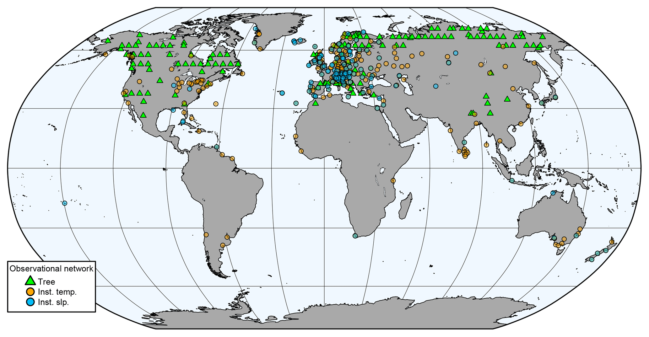
Figure 1The observational network in 1904, before the quality check.
2.3 Assimilation method
In our paleoclimate reconstruction, we combine the CCC400 model simulation with the observations as described above by implementing a modified version of the ensemble square root filter (EnSRF; Whitaker and Hamill, 2002). This ensemble-based DA method is called ensemble Kalman fitting (EKF; Franke et al., 2017a). In fact, the EKF is an offline version of the EnSRF, and the update step of the EKF remains the same as of the EnSRF. EKF is described in more detail in Bhend et al. (2012) and Franke et al. (2017a). Here, we shortly highlight the most important aspects of the EKF. The update step in the EnSRF scheme has two parts: updating the mean (), and for each member, the deviation from the mean (x′). They are calculated as
where K and are
The background state vector (xb) contains the variables of interest from CCC400 (Table 1). In the EKF, the length of the assimilation window is 6 months (October–March and April–September), which was adapted to the Southern and Northern Hemisphere growing seasons to effectively incorporate the proxy records stored in trees. Due to the 6-monthly assimilation window, xb contains the variables of 6 months. xa stands for the analysis state vector. H is the forward operator that maps the model state to the observation space (here, it is linear). H differs depending on the type of observation being assimilated. In the case of tree-ring width data, H extracts temperature between May and August and precipitation between April and June from the model; these fields are transformed to observational space by using a multiple regression approach (for more details, see Franke et al., 2017a). y represents the observations. K is the Kalman gain matrix, and is the reduced Kalman gain matrix. Pb is the background-error covariance matrix, estimated from the 30 ensemble members. A common assumption is to treat the observation-error covariance matrix (R) as a diagonal matrix: it is presumed that the elements of R are uncorrelated. Therefore, the observations can be processed serially. We set the error variances of instrumental temperature observations to 0.9 K2 and of instrumental pressure data to 10 hPa2. The error variances are rough estimates that include, for instance, measurement uncertainties, temporal inhomogeneities and the fact that a station is not representative for a grid cell (see Frei, 2014; Franke et al., 2017a). The errors of tree-ring proxy data are calculated as the variance of the multiple regression residuals of the H operator. The assimilation is conducted on the anomaly level: we subtract both from model and from observational data their 71-year running mean in order to deal with the biases related to systematic model errors and inconsistent low-frequency variability in the paleoclimate data.
The use of DA in an offline manner is typical in paleoclimate reconstructions (e.g., Dee et al., 2016). Bhend et al. (2012) argue that the assimilation step is too long for initial conditions to matter, whereas there is some predictability from the boundary conditions. In addition, Matsikaris et al. (2015) found that both online and offline DA methods perform similarly in their paleoclimate reconstruction setup. Furthermore, the offline DA is advantageous as it allows using the precomputed simulations. In our case, we can use CCC400 (Bhend et al., 2012) and test the method without having to repeat the simulations.
2.4 Spatial localization
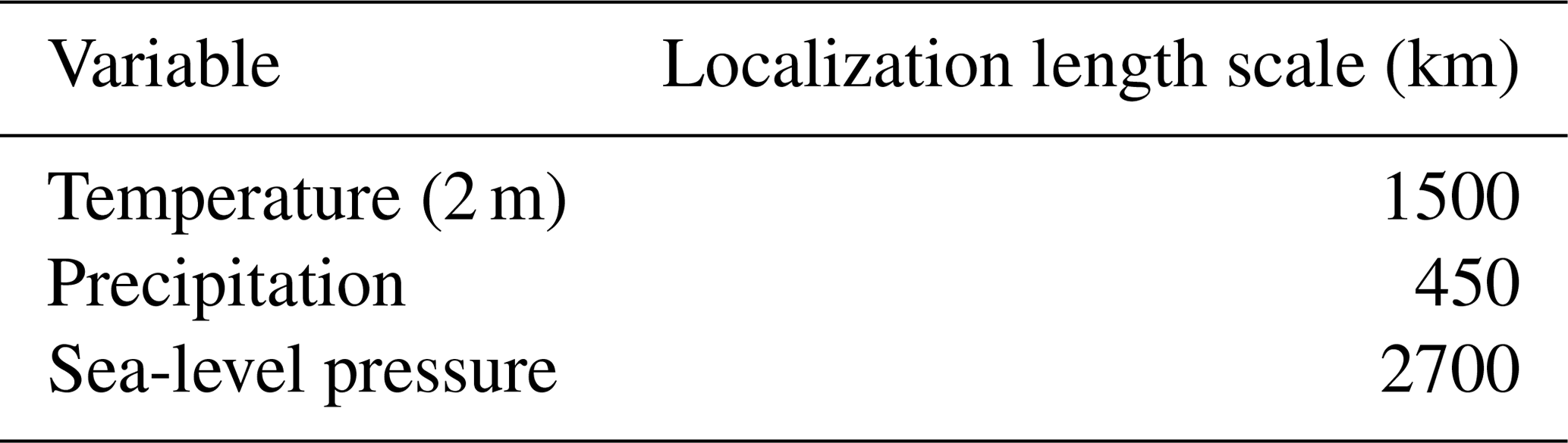
As R is a diagonal matrix, the EKF can be used to assimilate the observations one by one; that is, after the first observation is assimilated and the analysis is obtained, this analysis field becomes the background state for the next observation (see the arrow pointing from xa to xb on Fig. 2). This serial implementation makes the calculation of Pb simpler. H becomes a vector (not a matrix) of the same length as xb. It is zero everywhere except for a few elements (those required to model the observation). This translates to only a few columns of Pb that are actually required. HPbHT and R are then scalars (Whitaker and Hamill, 2002). This procedure also makes the localization simpler, as it needs to be applied only to those columns. In the original setup, the elements of Pb were multiplied (Schur product) with a distance-dependent function (see Eq. 7 in Franke et al., 2017a). For all the variables in the state vector, the same Gaussian function was used but with different localization length scale parameters (Table 1). The localization length scale parameters are defined based on the spatial correlation of the variables in the monthly CCC400 model simulation fields. For the cross-covariances between two variables, the smaller localization length scale of the two variables is applied. With the serial implementation, the calculation and localization of Pb is significantly simplified.
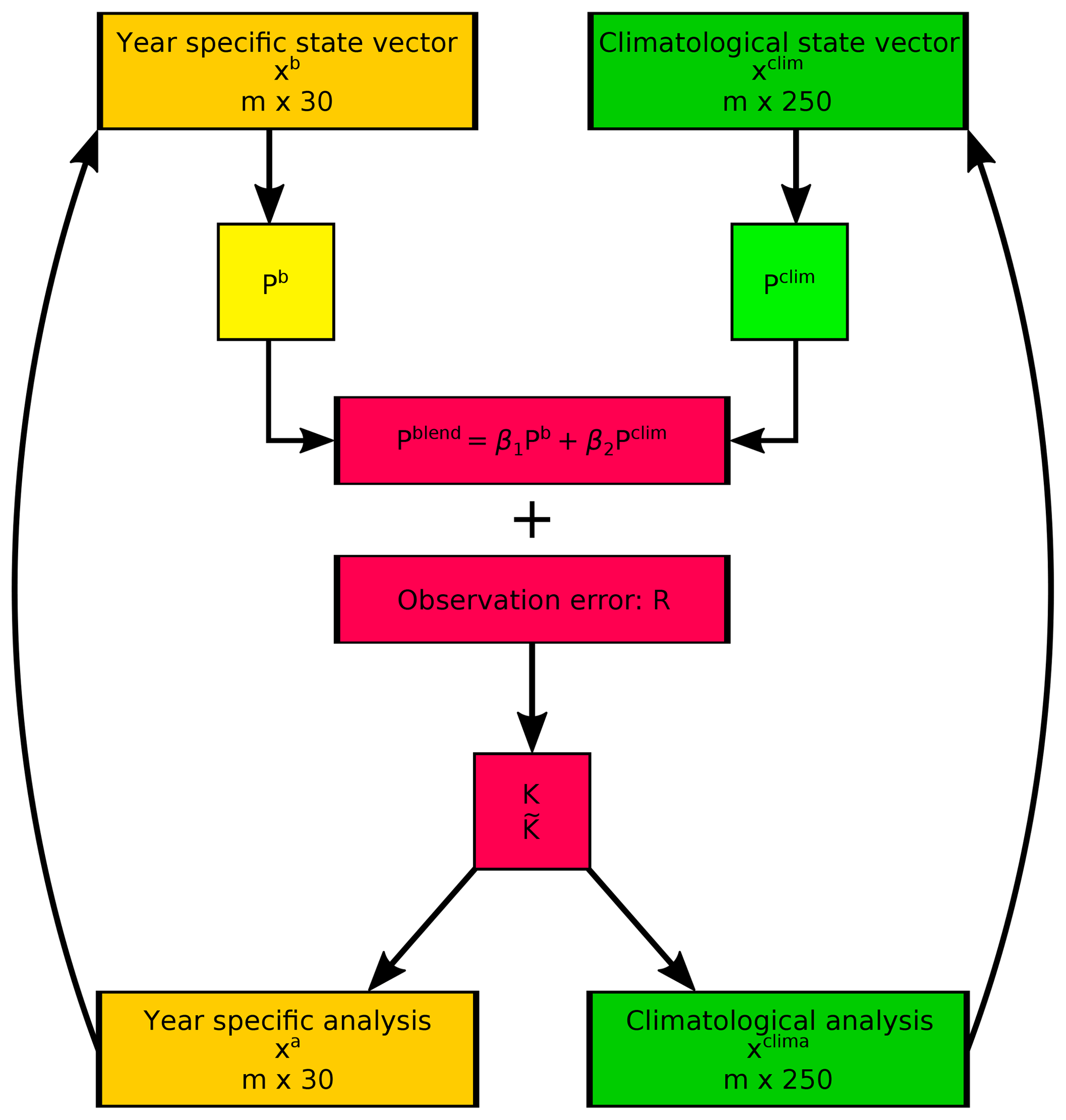
Figure 2The main steps of the blending experiment in one assimilation window. The blended covariance matrix Pblend is calculated as a linear combination from the year specific and climatological covariance matrices. The calculation of the Kalman gain (K) and reduced Kalman gain () matrices is the same as in Eqs. (3) and (4) except the covariance matrix is replaced with Pblend. The observation is assimilated to both state vectors and these analysis become to the starting point for assimilating the next observation.
Franke et al. (2017a) produced a monthly global paleoclimatological data set by using the EKF method. We leave most of the original setup unchanged and mainly focus on the estimation of Pb. To investigate the performance of the EKF, some aspects involving localization and estimation of the Pb were tested. An overview of all experiments conducted in this study is given in Table 2. The results of the various experiments are evaluated in terms of performance measures, which then compared to those obtained with the original setup.
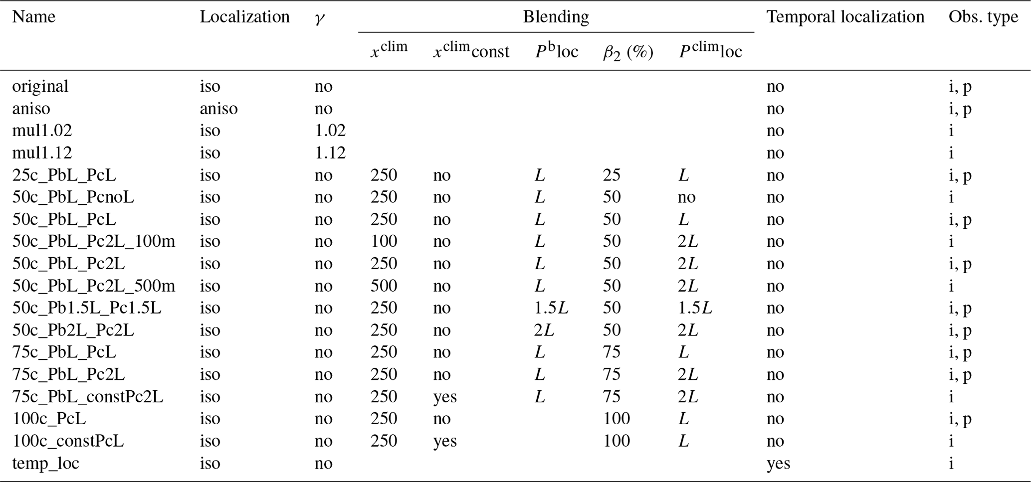
Table 2Summary of the experiments carried out in this study. The names of the experiments indicate which settings were used in the assimilation. Localization refers to the shape of the localization function applied on Pb. γ is the multiplicative inflation factor. xclim indicates from how many ensemble members the climatological state vector was constructed. xclimconst stands for keeping the climatological part in the blending experiment unchanged in one October–September time window. Pbloc indicates the localization length scale parameter applied for localizing Pb. β2 refers to the weight given to Pclim. Pclimloc indicates the localization length scale parameter applied for localizing Pclim. i and p stand for instrumental-only and proxy-only observation experiments, respectively.
3.1 Spatial localization
In most of the studies, the localization function is implemented in an isotropic manner. In the original setup, the same horizontally isotropic localization function was used with different localization parameters. However, such spatial symmetries may not be realistic. In the real atmosphere, correlation lengths might be longer in the zonal than in the meridional direction, due to the prevailing winds and the weaker large-scale temperature gradients in this direction. On multi-annual to multi-decadal timescales, multiple processes act in the meridional direction, e.g., a widening/shrinking of the Hadley cell, shifts of the Intertropical Convergence Zone or changes in atmospheric modes like the Atlantic Multi-Decadal Oscillation or the North Atlantic Oscillation. These can shift the zonal circulation northward or southward, but the zonal coherence will be less effected. Hence, instead of using a circular Gaussian function, we conducted an experiment with a spatially anisotropic localization function
where dz and dm are the distances from the selected grid box in the zonal and meridional directions, respectively. Lz and Lm are the length scale parameters used for localization in the zonal and meridional directions, respectively. As a first experiment, we tested a 2:1 ratio for Lz:Lm. We used the values from Table 1 in the meridional direction and doubled them in the zonal direction. Thus, the resulting localization function has an elliptical shape.
3.2 Inflation techniques
Covariance inflation techniques are another possible method to compensate for errors in the DA system (Whitaker et al., 2008). The multiplicative inflation technique uses a small factor γ(γ>1) with which the x′b is multiplied (Anderson and Anderson, 1999). This type of covariance inflation accounts for filter divergence due to sampling error (Whitaker and Hamill, 2002) but can be also applied to take into account system errors (Whitaker et al., 2008). We conducted some experiments using multiplicative inflation, although in our offline approach, filter divergence is not the main concern as ensemble members are not propagated in time.
The other methodology that we adapt shows similarities with the additive inflation technique (e.g., Houtekamer and Mitchell, 2005) and with the hybrid DA scheme (e.g., Clayton et al., 2013). In both methods, Pb is modified by either adding model error (Houtekamer and Mitchell, 2005) or a so-called climatological covariance matrix (Clayton et al., 2013) to Pb. This has given rise to the idea of generating a climatological ensemble in order to alleviate the effect of the small ensemble size. In the original setup, Pb is approximated from only 30 members. Here, we additionally build a climatological state vector (xclim) from randomly selected ensemble members from our 400-year long model simulation. The number of ensemble members should be higher than the original ensemble size, but still computationally affordable. The climatological state vector is created as follows: (1) define the ensemble size (n) of xclim; (2) select n random years between 1601 and 2005; (3) every year has 30 members from which one member is randomly selected and kept; (4) the chosen members are combined in xclim. xclim is randomly resampled after every second assimilation cycle. Using xclim in the assimilation leads to increased computational cost, which partly comes from the creation of xclim. The other time-consuming part comes from the updating of the climatological part after each observation is assimilated (the standard way when observations are assimilated serially). We tested numbers between 100 and 500. From xclim, a climatological background-error covariance matrix (Pclim) can be obtained by using the ensemble perturbations. The background-error covariance matrix used in the blending experiments (Pblend) is built as a linear combination of the sample covariance matrix (Pb) and the climatological covariance matrix (Pclim):
where β1, β2 are the weights given to the covariance matrices. The sum of the weights is unity.
Figure 2 shows the main steps of the blending assimilation process. First, the covariance matrices were localized separately; then, we blended them according to the given weights. We conducted several experiments to tune the ratio between the two covariance matrices while using different localization length scale parameters (L) (Table 2). We used the same L values for localizing Pb in most of our experiments to evaluate improvements in comparison with the original setup. For this study, we calculated the latitudinal dependency of correlation of the state variables from a bigger ensemble of the model than in Franke et al. (2017a). The result suggested that longer L values can be applied in the tropics and the L of precipitation is probably too strict. Based on the rather strict L values in the previous study and the assumption that the covariances can be better estimated from a bigger ensemble, we used doubled length scale parameters (2L) in some of the experiments for localizing the climatological covariances. In this case, the L for temperature is 3000 km, which means that the correlation is decreased close to zero approximately 6000 km away from the observation.
Since observations are assimilated serially, we also update xclim after an observation is assimilated with the same Kalman gain matrices as xb. Thus, in the assimilation process, we update 30+n ensemble members.
3.3 Temporal localization
Localizing observations in time is a special feature of the EKF due to its 6-month assimilation window. Having the state vector in half-year format, every month within the October–March or April–September time window is updated by each single observation. To test whether the covariances between a single observation and the multivariate climate fields are correctly captured, we ran an instrumental-only experiment with temporal localization. We set covariances between different months to zero.
3.4 Skill scores
The EKF method is tested with different localization functions and with a set of mixed background-error covariance matrices as described above. We have performed the experiments by assimilating either only proxy records (proxy-only experiment) or only instrumental data (instrumental-only experiment). The proxy-only experiments were carried out between 1902 and 1959, because many proxy records already end in the 1960s, while the instrumental-only experiments were tested over the 1902–2002 period. We separated the different observation types to see whether different settings perform better depending on the type of data being assimilated. We do not compare proxy-only results with instrumental-only results; hence, the difference in time periods used does not matter; we simply use the longest possible time period. To evaluate the reconstructions, we examined two verification measures: correlation coefficient and reduction of error (RE) skill score (Cook et al., 1994). We use the Climate Research Unit (CRU) TS 3.10 dataset (Harris et al., 2014) for reference in the validation process. The presented verification measures are functions of time. Correlation is calculated between the absolute values of the ensemble mean of the analysis and the reference series at each grid point. The RE compares, in our case, the reconstruction with the model simulation, both expressed as deviations from a reference.
where xu is the ensemble mean of the analysis, xf is the ensemble mean of the model background state, xref is the reference dataset, and i refers to the time step. The RE skill scores are computed based on anomalies with respect to the 71-year running climatologies. Note that xf comes from a forced model simulation; therefore, it already has skill compared with a climatological state vector. The RE is 1 if the xu is equal to xref. Negative RE values indicate that the background state is closer to the reference series than the analysis.
To test which experiments have significantly different skill compared with the original skill, we carried out a permutation test following the method described in DelSole and Tippett (2014). Permutation was performed 10 000 times. If the difference between the median of the experiment and the median of the original data falls outside of the 95 % confidence level of the interval calculated from permuted data, then the experiment is significantly different from the original data.
In the next section, we will focus on analyzing the result of the experiments mainly over the extratropical Northern Hemisphere (ENH), because most of the data are located in this region. The skill scores refer to seasonal averages of the ensemble mean.
4.1 Localization function
4.1.1 Results
We compared the original setup applying an isotropic localization function and the experiment in which an anisotropic localization function was used, to test whether we can obtain a more skillful reconstruction by implementing anisotropic localization method. As an example of the spatial reconstruction skill, we show the RE values of temperature (Fig. 3). The figures reveal that the type of localization function only resulted in small differences in both experiments. Nonetheless, there are larger areas of negative RE values (Greenland, Siberia) with the anisotropic localization function in the proxy-only experiment (Fig. 3). In the instrumental-only experiment, the decrease of RE values occur in the northern high latitudes and in the Tibetan Plateau in both seasons (Fig. 3). To have a better overview of how the skill scores changed, we summarize their distributions with the help of box plots. Figure 4 shows the differences of skill scores between the aniso experiment and the original skill for the three variables (temperature, precipitation and sea-level pressure) in the ENH region. In the instrumental-only experiment, correlation values of temperature and sea-level pressure decreased in both seasons, while for precipitation they remained mostly unchanged. The RE values show that the experiments with anisotropic localization function reduced the skill of the reconstructions, but the extent of the reduction varies with the variables and with the seasons (Fig. 4). In general, the same holds for the proxy-only experiment (Fig. 4).
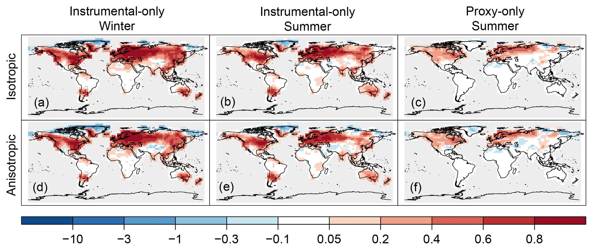
Figure 3Spatial skill of temperature reconstruction presented by RE values, assimilating only instrumental data (a, b, d, e) and only proxy records (c, f). Comparing the skill of the reconstruction using isotropic localization function (a–c) versus an anisotropic localization function (d–f). Skill in the winter season (a, d) and in the summer season (b, e, c, f) are shown.
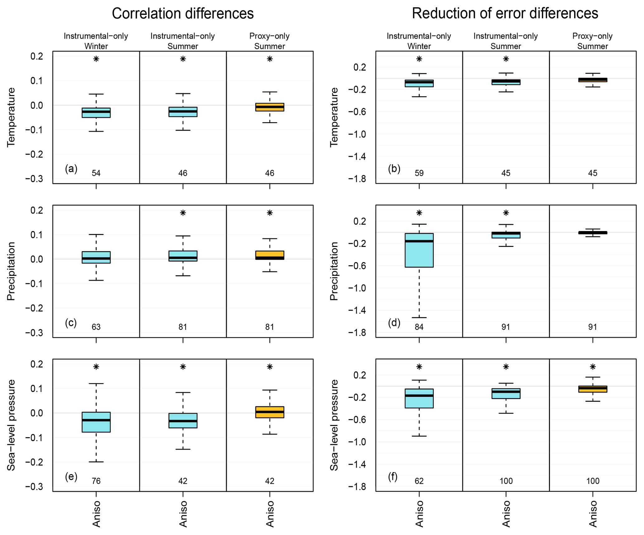
Figure 4Difference between the aniso experiment and the original setup in terms of skill scores over the ENH region. Distributions of correlation values and of RE values are on the left and right figures, respectively. Distribution of temperature (a, b), precipitation (c, d) and sea-level pressure (e, f) are shown. Blue color indicates the instrumental-only experiment and yellow indicates the proxy-only experiment. The midline of the box is the median. The lower (upper) border of the box is the first (third) quartile. The whiskers extend up to 1.5 times the interquartile range; beyond these distances, the number of outliers is given under the box plots. The grid boxes were not area weighted. The asterisk above the box indicates significant differences between the median of the experiment and the original setup.
4.1.2 Discussion
In a previous ozone reconstruction study, a seasonally and latitudinally varying localization method was tested which mostly positively affected the analysis (Brönnimann et al., 2013). Here, we increased the zonal distances to see if we can use the information of the observations for a larger region. However, the verification measures are shifted more to the negative direction. We assume that the degraded skill of the reconstruction is due to the choice of too-long Lz; hence, spurious correlations were not removed. Using anisotropic localization (doubling the L values only in the zonal direction) consistently makes the reconstruction worse.
4.2 Inflation experiments
4.2.1 Results
The main problem of ensemble-based DA techniques is the computationally affordable limited ensemble size. Due to the finite ensemble size, the estimation of Pb suffers from sampling error. Applying inflation techniques is one method to mitigate its effect (see Sect. 3.2).
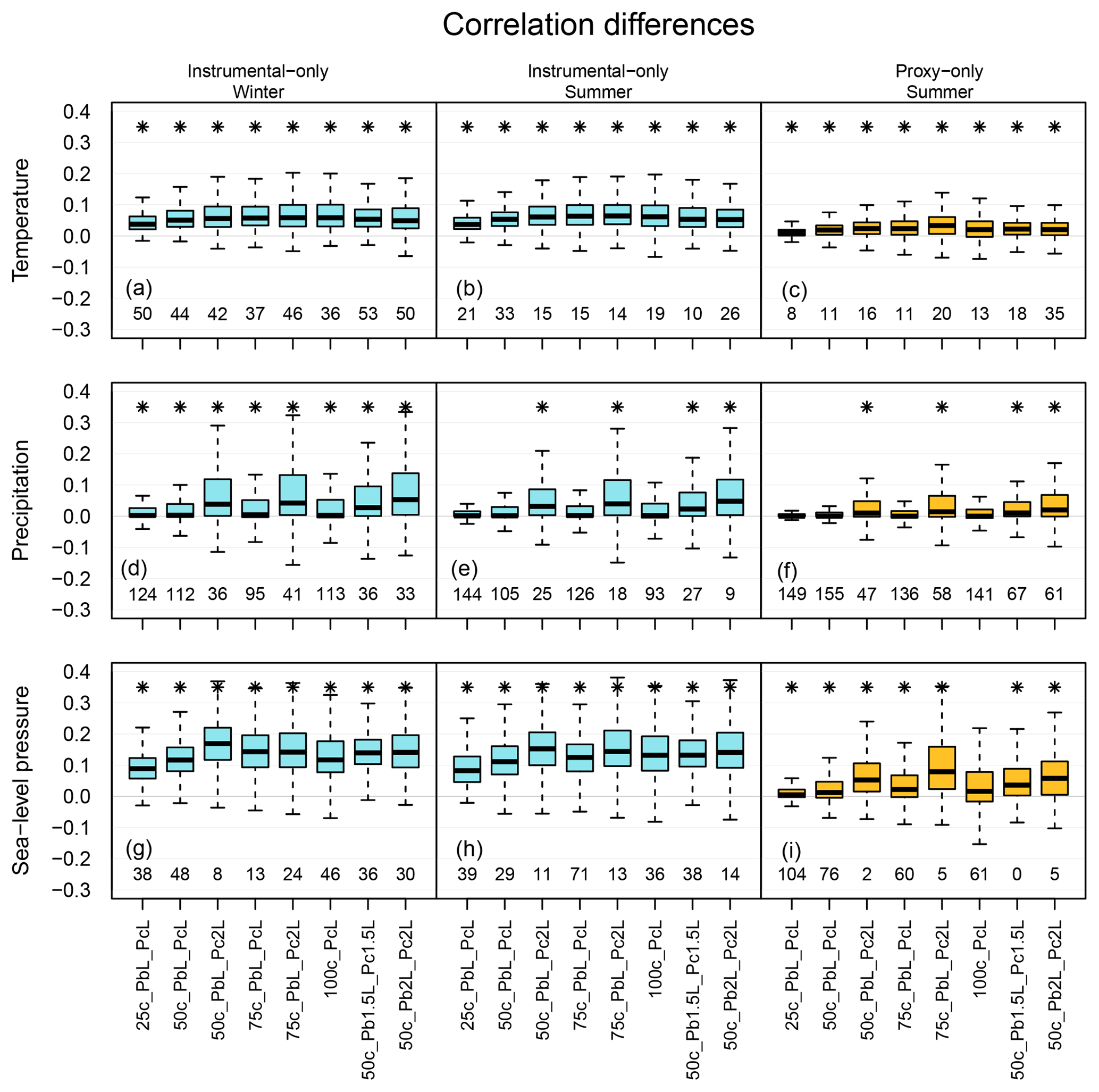
Figure 5Distribution of correlation coefficients differences between the mixed background-error covariance matrix experiments and the original setup over the ENH region. Panels (a), (d) and (g) show the skill of the reconstruction in the winter seasons, while panels (b), (c), (e), (f), (h) and (i) show it for the summer season. The labels on the x axis indicate the experiments. Box plot, color, number and asterisk are the same as in Fig. 4.
Using the multiplicative inflation method, the deviations from the ensemble mean are multiplied with a small factor (γ). To find the optimal γ, a set of experiment runs is required. We used γ=1.02 and γ=1.12 in our experiments, where only instrumental data were assimilated. We chose γ from a range that was previously tested by Whitaker and Hamill (2002). Multiplying the deviations from the ensemble mean with γ=1.02 in the assimilation process hardly affected the skill of the reconstruction over the ENH region (not shown). When we increased the value of γ to 1.12, the RE values slightly decreased (not shown). We did not carry out further experiments since, based on the results, randomly increasing the error in background field did not lead to improvement.
In the other set of experiments, we used Pblend in the update equation (Eq. 6). The experiments were run with using β2 equal to 0.25, 0.50, 0.75 and 1 to estimate the Pblend (denoted 25c, 50c, etc.). Besides the varying weight given to Pclim, the applied L values on Pb and Pclim differed as well. Three L values were used: no localization (termed “no”), applying L values as in Table 1 (L) and doubling these numbers (2L). Different combinations of the fraction of Pclim and L values were termed accordingly (e.g., 50c_PbL_Pc2L).
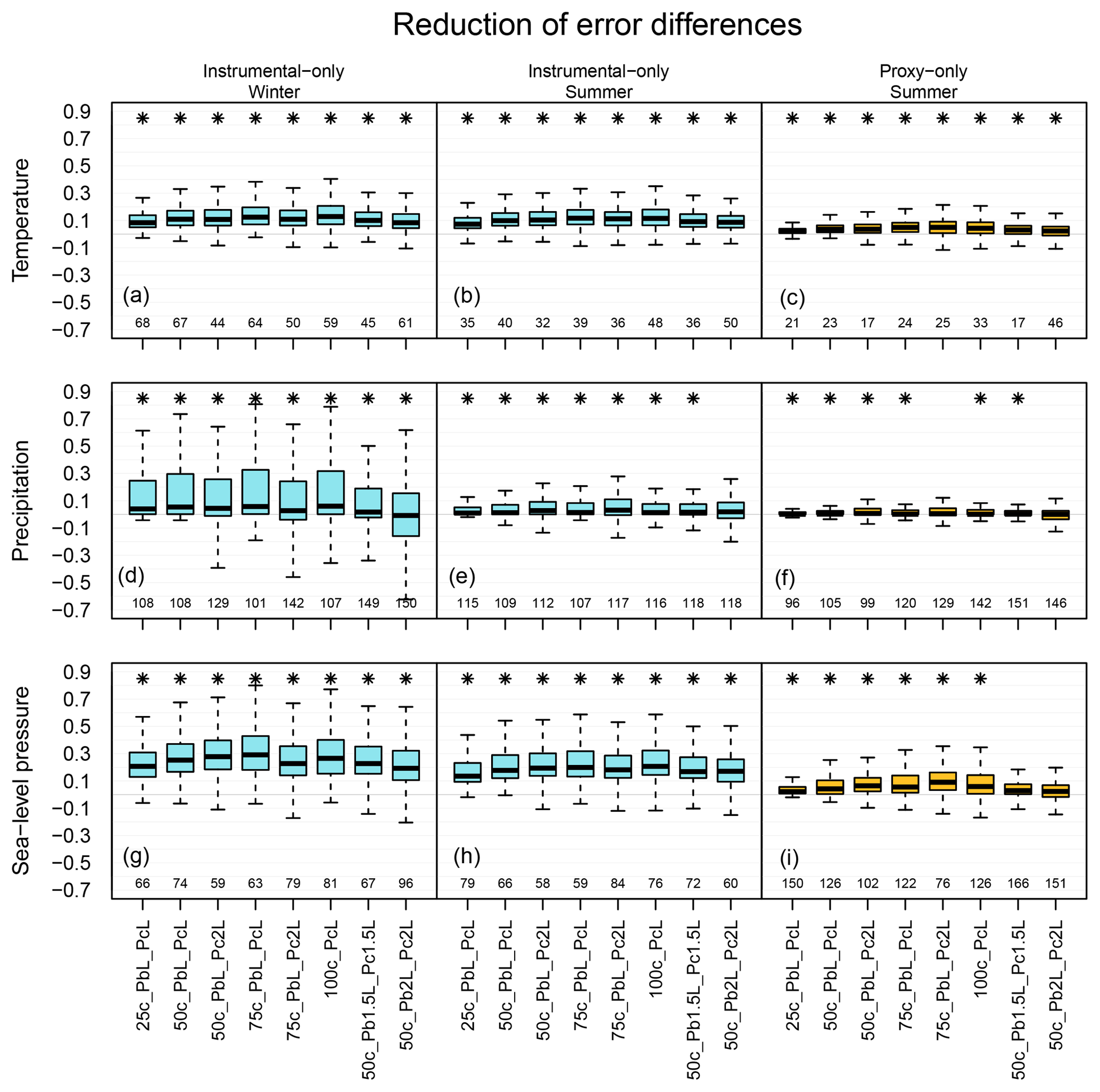
Figure 6Distribution of RE value differences between the mixed background-error covariance matrix experiments and the original setup over the ENH region; otherwise, it is the same as in Fig. 5.
We expect that estimating the covariances from a bigger ensemble size (n = 100–500) instead of 30 members leads to a more accurate background matrix. In most of our experiment, n is 250. Hence, Pclim is likely less affected by the sampling error implying that long-range spurious correlations are less prominent, which makes localization less needed. We presume that using Pblend helps to better reconstruct areas which were characterized with lower skill score values in the original setup and to improve the estimation of unobserved climate variables. The reconstruction skill of the blending experiments is always calculated from xa (Fig. 2).
For the ENH region, we present how the verification measures changed by replacing Pb with Pblend in the assimilation process. We conducted an experiment without localizing Pclim and using L values from Table 1 on Pb in the construction of Pblend. However, the skill of the reconstruction was largely reduced, implying that 250 members are not enough to avoid localization altogether (not shown).
Figures 5 and 6 show the distribution of the differences of the skill scores between the experiments and the original analysis for correlation coefficients and RE values, respectively. Depending on the variables and the data type being assimilated, different setups perform better. In the case of assimilating only instrumental data, one of the largest increases of median for temperature reconstruction was obtained from the 100c_PcL experiment in both seasons (Figs. 5, 6). Precipitation records were not assimilated; thus, a reasonable estimation of the cross-variable covariances is essential. The skill of the precipitation reconstruction with the original setup, in terms of correlation, is better than the forced simulation (not shown); however, the RE values are negative over large regions in the ENH (Fig. 7). Using Pblend in the assimilation, with, e.g., the settings of 50c_PbL_Pc2L experiment, led to more positive RE skill (Fig. 7). The biggest improvement, in terms of RE skill score, was found in Europe (Fig. 7). The 50c_PbL_Pc2L analysis also has higher skill in North-America, especially in the summer season (Fig. 7). The skill of the sea-level pressure reconstruction also improved in the 50c_PbL_Pc2L experiment (Figs. 5, 6). In the proxy-only experiments, 75c_PbL_Pc2L is among the best performing experiments for all the variables (Figs. 5, 6).
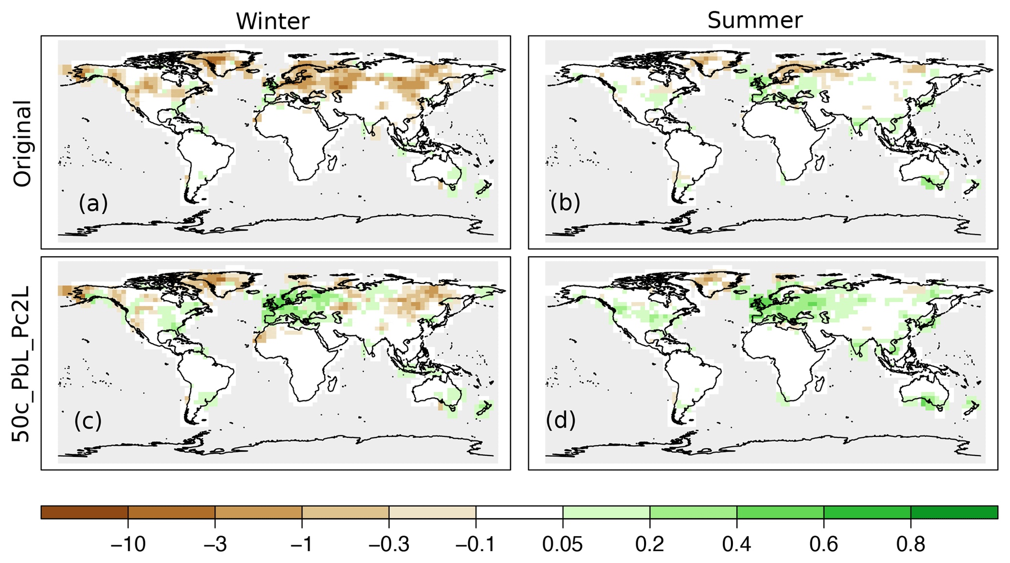
Figure 7Spatial reconstruction skill of precipitation in terms of RE values, assimilating only instrumental data. Panels (a) and (b) show the skill of the original setup, and (c) and (d) show the result of the 50c_PbL_Pc2L experiment. The skill in the winter season is presented in panels (a) and (c), and for the summer season in panels (b) and (d).
We also investigated the effect of the ensemble size in the estimation of Pclim. To test whether further improvements can be achieved by doubling the ensemble size of xclim, we ran an experiment with the following setup: β1 and β2 are equally weighted, and L and 2L are applied on Pb and Pclim, respectively (Table 2). In the experiment, we assimilated only instrumental data. The skill scores of xa (corr, RE) from the 500-ensemble-member experiment showed no marked improvement compared with the same experiment with 250 ensemble members. An additional experiment was carried out with the same setup but using only 100 ensemble members in the construction of xclim. The verification measures of the 50c_PbL_Pc2L_100m experiment are higher than the original one, and the distribution of the skill scores over the ENH region is very similar to what we obtain by using 250 members in Pclim for temperature and precipitation. However, the sea-level pressure fields from the 50c_PbL_Pc2L experiment have higher skill than those in the 50c_PbL_Pc2L_100m experiment (not shown).
Furthermore, we conducted two experiments in which only xb was updated after an observation was assimilated, and xclim was kept constant in the assimilation window. However, the ensemble members of xclim were randomly reselected for each year (October–September). The advantage of this setup compared to the setup described in Sect. 3.2 is that it is computationally less demanding since only the original 30 members keep being updated with the observations. In the first test, we give β2=0.75 weight to Pclim with 2L values. In the second test, β2=1; that is, only Pclim used for updating xb and the L values in Table 1 were applied for the localization. By comparing the skill of the reconstructions without and with updating the climatological part, we see that the skill scores are higher when the climatological part is also updated with the information from the observations (Fig. 8). The only exception is the correlation values of sea-level pressure: when keeping the climatological part constant, they are slightly higher in both seasons (Fig. 8). Nonetheless, by keeping the climatological part static in one assimilation window, the experiments still outperform the original reconstruction (Fig. 8).
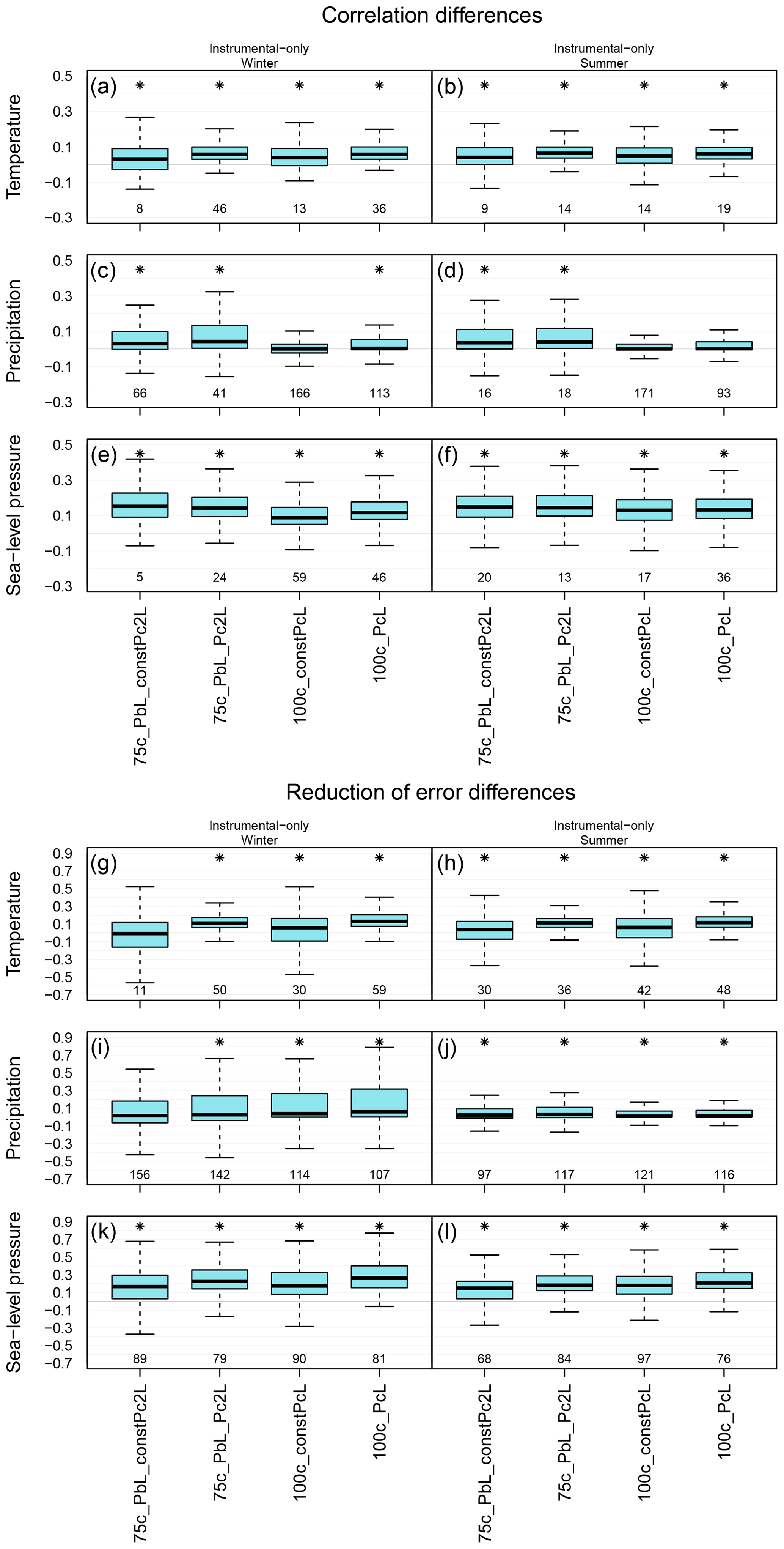
Figure 8Distribution of skill scores over the ENH region. The skill of the original setup is compared with experiment 75c_PbL_constPc2L, 75c_PbL_Pc2L, 100c_constPcL and 100c_PcL. Distribution of correlation coefficients in the winter (left column) and in the summer (right column) seasons. Distribution of RE values in the winter (left column) and in the summer (right column) seasons.
4.2.2 Discussion
We have tested a number of configurations of the mixed covariance matrix Pblend to evaluate the effect of the sampling error. In numerical weather predication (NWP) applications, various methods have been designed to better estimate the errors of the background state. In hybrid DA systems, the advantages of variational and ensemble Kalman filter techniques are combined (Hamill and Snyder, 2000; Lorenc, 2003). In another method, the background-error covariances are obtained from an ensemble of assimilation experiments performed by a variational assimilation system (Pereira and Berre, 2006). In an additive inflation experiment, a term is added to the xa to account for the errors of the DA system (Whitaker et al., 2008).
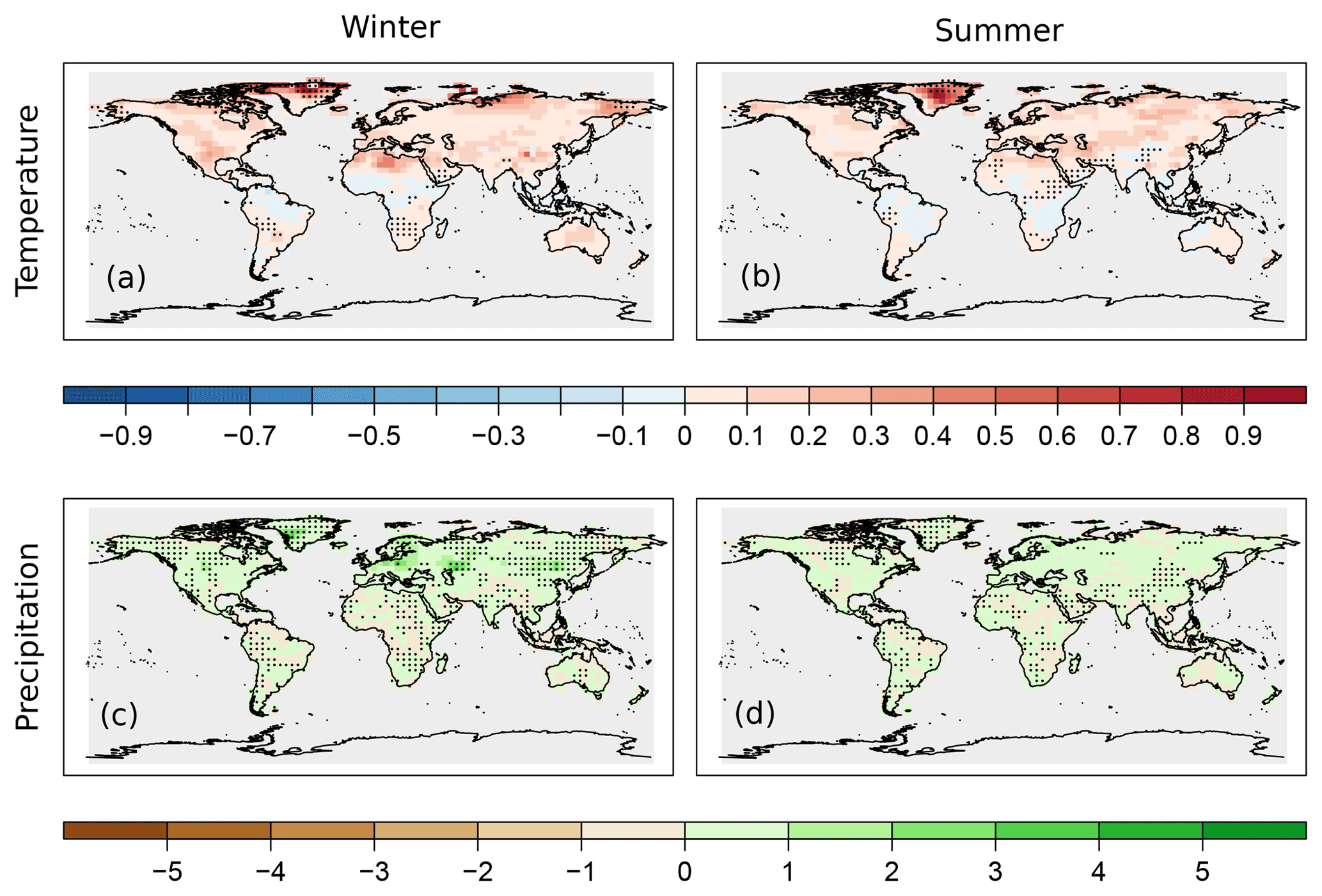
Figure 9Difference of the RE skill between the temporally localized experiment and the original setup, when only instrumental data are assimilated. Temperature (a, b) and precipitation (c, d) differences are shown in the winter (a, c) and in the summer (b, d) seasons. The black dots indicate the negative RE values in the temporally localized experiment.
In our implementation, Pblend is calculated from xb and xclim. Using Pblend in the assimilation process improved on the reconstruction performed with the original setup. The skill scores show the largest improvement in the sea-level pressure reconstruction. Moreover, the skill of the precipitation reconstruction also improved, indicating that Pclim helps to better estimate the cross-covariances of the background errors between the variables. In general, increasing the weight of Pclim in forming Pblend positively affected the skill of the analysis. The 100c_PcL experiment, in which Pblend is equal to Pclim, is similar to the DA technique used in the last millennium climate reanalysis (LMR) project (Hakim et al., 2016). In the LMR, 100 randomly chosen ensemble members form a climatological state vector, which is used in each assimilation window and is updated with the observations. In this study, xclim is randomly resampled every year and primarily used in the estimation of Pblend. The settings used in the 100c_PcL experiment led to one of the largest increases in the median for temperature reconstruction when only instrumental measurements are assimilated. However, other settings resulted in larger increase of median for different variables and observation types. By applying no localization on Pclim in the 50c_PbL_PcnoL experiment, we obtained a less skillful reconstruction than by using the other two localization schemes. The skills reduced especially over the areas where no local observations were assimilated. Using 2L values for localizing the covariances of Pclim in the instrumental-only experiments resulted in higher correlation values of sea-level pressure (50c_PbL_Pc2L) and helped to obtain higher correlation scores of precipitation in summer. Among the proxy-only experiments, 75c_PbL_Pc2L shows the largest increase of median for pressure reconstruction. Here, pressure data are not assimilated, and the result suggests that by applying longer L values, the cross-variable covariances are treated better. We tested whether the skill of the experiments performed with various settings is significantly different from the skill of the original analysis. We compared the median value of the skill scores from the experiments and the original data, and with most of the settings a significant difference was obtained for all the variables. The results of the experiments show that with a mixed covariance matrix implementation, a major drawback of the ensemble-based DA system, due to the limited ensemble size, can be improved.
4.3 Localization in time
4.3.1 Results
Since 6-monthly time steps were combined in one state vector (one assimilation window), covariances between different months also need to be considered. An additional experiment was conducted in which the (localized) Pb was multiplied with a temporal localization function when instrumental data were assimilated. This is a specific experiment due to the structure of EKF. The assimilation window in the EKF is 6 months; hence, a single observation is enabled to adjust all the meteorological variables in xb in a half-year time window. In the temporal localization experiment, the information from a given observation can only modify the different climate fields in its current month, while leaving all other fields of the 5 months unchanged (Table 2). In general, the skill scores indicate an improvement. The differences of RE values between the temp_loc and original experiments are mostly positive over the northern high-latitude areas (Fig. 9).
4.3.2 Discussion
The higher skill scores with temporal localization (Fig. 9) indicate that the cross-covariances in time were not correctly represented by Pb. Hence, it is likely that in the original setup some non-physical covariances were taken into account. Applying the same assimilation scheme to another problem (estimating the two-dimensional ozone distribution from an ensemble of chemistry–climate models and historical observations), Brönnimann et al. (2013) used a localization timescale of 3 months based on empirical studies. It may be worth considering or allowing for temporal covariance in specific cases (e.g., in the case of ozone concentrations) which vary on longer timescales.
In this study, a transient offline data assimilation approach was used to test the effect of the estimation of the background-error covariance matrix in a climate reconstruction. Several experiments were evaluated with different validation measures to see which background-error covariance matrix estimation techniques improve the skill of the reconstruction. The evaluation of the presented techniques suggests the following: (1) applying an anisotropic localization function on the sample covariance matrix did not improve the reconstruction; (2) most of the settings, which make use of covariance estimates from a larger climatological sample, result in significantly improved skills compared to an estimation from the 30-member ensemble; (3) assimilating early instrumental data with temporal localization leads to a better analysis. To which extent the different techniques helped in the estimation of the background-error covariance matrix varies geographically and also depends on the climate variable being reconstructed. The cross-variable covariances of the background-error covariance matrix can provide information from unobserved climate variables. Including climatological information in the estimation of precipitation has led to a better reconstruction, especially in Europe. Estimating sea-level pressure with the blended Pblend matrix also improved the skill of the reconstruction. For instance, the 50c_PbL_Pc2L experiment performs constantly better than the original setup. This study shows that results can be improved by better specifying the background-error covariance matrix. In the future, we will combine all the techniques that lead to more skillful analyses to produce a climate reconstruction over the last 400 years.
The EKF400 reanalysis is available at the World Data Center for Climate at Deutsches Klimarechenzentrum (DKRZ) in Hamburg, Germany (https://cera-www.dkrz.de/WDCC/ui/cerasearch/entry?acronym=EKF400_v1.1; Franke et al., 2017b). The sensitivity experiments analyzed in this study are available upon request: veronika.valler@giub.unibe.ch, joerg.franke@giub.unibe.ch.
All authors were involved designing the study and contributed to writing the paper. VV conducted the experiments and performed most of the analyses. JF developed the original code and helped with the analyses.
The authors declare that they have no conflict of interest.
The CCC400 simulation was performed at the Swiss National Supercomputing Centre CSCS. The comments of the two anonymous reviewers are gratefully acknowledged.
This research has been supported by the Swiss National Science Foundation (grant no. 162668) and the European Commission – Horizon 2020 (grant no. 787574).
This paper was edited by Bjørg Risebrobakken and reviewed by two anonymous referees.
Anderson, J. L. and Anderson, S. L.: A Monte Carlo implementation of the nonlinear filtering problem to produce ensemble assimilations and forecasts, Mon. Weather Rev., 127, 2741–2758, https://doi.org/10.1175/1520-0493(1999)127<2741:AMCIOT>2.0.CO;2, 1999. a, b, c, d
Bhend, J., Franke, J., Folini, D., Wild, M., and Brönnimann, S.: An ensemble-based approach to climate reconstructions, Clim. Past, 8, 963-976, https://doi.org/10.5194/cp-8-963-2012, 2012. a, b, c, d, e, f, g
Bowler, N., Clayton, A., Jardak, M., Jermey, P., Lorenc, A., Wlasak, M., Barker, D., Inverarity, G., and Swinbank, R.: The effect of improved ensemble covariances on hybrid variational data assimilation, Q. J. Roy. Meteor. Soc., 143, 785–797, https://doi.org/10.1002/qj.2964, 2017. a
Brönnimann, S., Bhend, J., Franke, J., Flückiger, S., Fischer, A. M., Bleisch, R., Bodeker, G., Hassler, B., Rozanov, E., and Schraner, M.: A global historical ozone data set and prominent features of stratospheric variability prior to 1979, Atmos. Chem. Phys., 13, 9623–9639, https://doi.org/10.5194/acp-13-9623-2013, 2013. a, b
Clayton, A. M., Lorenc, A. C., and Barker, D. M.: Operational implementation of a hybrid ensemble/4D-Var global data assimilation system at the Met Office, Q. J. Roy. Meteor. Soc., 139, 1445–1461, https://doi.org/10.1002/qj.2054, 2013. a, b
Cook, E. R., D'Arrigo, R., and Anchukaitis, K.: ENSO reconstructions from long tree-ring chronologies: Unifying the differences?, talk presented at a special workshop on “Reconciling ENSO Chronologies for the Past 500 Years”, 2–3 April 2008, Moorea, French Polynesia, 2008. a
Cook, E. R., Briffa, K. R., and Jones, P. D.: Spatial regression methods in dendroclimatology: a review and comparison of two techniques, Int. J. Climatol., 14, 379–402, https://doi.org/10.1002/joc.3370140404, 1994. a
Dee, S. G., Steiger, N. J., Emile-Geay, J., and Hakim, G. J.: On the utility of proxy system models for estimating climate states over the common era, J. Adv. Model. Earth Sy., 8, 1164–1179, https://doi.org/10.1002/2016MS000677, 2016. a
DelSole, T. and Tippett, M. K.: Comparing forecast skill, Mon. Weather Rev., 142, 4658–4678, https://doi.org/10.1175/MWR-D-14-00045.1, 2014. a
Franke, J., Brönnimann, S., Bhend, J., and Brugnara, Y.: A monthly global paleo-reanalysis of the atmosphere from 1600 to 2005 for studying past climatic variations, Scientific data, 4, 170076, https://doi.org/10.1038/sdata.2017.76, 2017a. a, b, c, d, e, f, g, h, i, j, k, l, m, n
Franke, J., Brönnimann, S., Bhend, J., and Brugnara, Y.: Ensemble Kalman Fitting Paleo-Reanalysis Version 1.1, World Data Center for Climate (WDCC) at DKRZ, available at: http://cera-www.dkrz.de/WDCC/ui/Compact.jsp?acronym=EKF400_v1.1 (last access: 19 July 2019), 2017b. a
Frei, C.: Interpolation of temperature in a mountainous region using nonlinear profiles and non-Euclidean distances, Int. J. Climatol., 34, 1585–1605, 2014. a
Gaspari, G. and Cohn, S. E.: Construction of correlation functions in two and three dimensions, Q. J. Roy. Meteor. Soc., 125, 723–757, https://doi.org/10.1002/qj.49712555417, 1999. a
Gebhardt, C., Kühl, N., Hense, A., and Litt, T.: Reconstruction of Quaternary temperature fields by dynamically consistent smoothing, Clim. Dynam., 30, 421–437, https://doi.org/10.1007/s00382-007-0299-9, 2008. a
Goosse, H., Renssen, H., Timmermann, A., Bradley, R. S., and Mann, M. E.: Using paleoclimate proxy-data to select optimal realisations in an ensemble of simulations of the climate of the past millennium, Clim. Dynam., 27, 165–184, https://doi.org/10.1007/s00382-006-0128-6, 2006. a
Goosse, H., Crespin, E., de Montety, A., Mann, M., Renssen, H., and Timmermann, A.: Reconstructing surface temperature changes over the past 600 years using climate model simulations with data assimilation, J. Geophys. Res.-Atmos., 115, D09108, https://doi.org/10.1029/2009JD012737, 2010. a
Hakim, G. J., Emile-Geay, J., Steig, E. J., Noone, D., Anderson, D. M., Tardif, R., Steiger, N., and Perkins, W. A.: The last millennium climate reanalysis project: Framework and first results, J. Geophys. Res.-Atmos., 121, 6745–6764, https://doi.org/10.1002/2016JD024751, 2016. a, b
Hamill, T. M. and Snyder, C.: A hybrid ensemble Kalman filter – 3D variational analysis scheme, Mon. Weather Rev., 128, 2905–2919, https://doi.org/10.1175/1520-0493(2000)128<2905:AHEKFV>2.0.CO;2, 2000. a
Hamill, T. M., Whitaker, J. S., and Snyder, C.: Distance-dependent filtering of background error covariance estimates in an ensemble Kalman filter, Mon. Weather Rev., 129, 2776–2790, https://doi.org/10.1175/1520-0493(2001)129<2776:DDFOBE>2.0.CO;2, 2001. a, b
Harris, I., Jones, P. D., Osborn, T. J., and Lister, D. H.: Updated high-resolution grids of monthly climatic observations–the CRU TS3. 10 Dataset, Int. J. Climatol., 34, 623–642, https://doi.org/10.1002/joc.3711, 2014. a
Houtekamer, P. L. and Mitchell, H. L.: Data assimilation using an ensemble Kalman filter technique, Mon. Weather Rev., 126, 796–811, https://doi.org/10.1175/1520-0493(1998)126<0796:DAUAEK>2.0.CO;2, 1998. a
Houtekamer, P. L. and Mitchell, H. L.: A sequential ensemble Kalman filter for atmospheric data assimilation, Mon. Weather Rev., 129, 123–137, https://doi.org/10.1175/1520-0493(2001)129<0123:ASEKFF>2.0.CO;2, 2001. a
Houtekamer, P. L. and Mitchell, H. L.: Ensemble Kalman filtering, Q. J. Roy. Meteor. Soc., 131, 3269–3289, https://doi.org/10.1256/qj.05.135, 2005. a, b
Houtekamer, P. L., Mitchell, H. L., Pellerin, G., Buehner, M., Charron, M., Spacek, L., and Hansen, B.: Atmospheric data assimilation with an ensemble Kalman filter: Results with real observations, Mon. Weather Rev., 133, 604–620, https://doi.org/10.1175/MWR-2864.1, 2005. a
Ide, K., Courtier, P., Ghil, M., and Lorenc, A. C.: Unified Notation for Data Assimilation: Operational, Sequential and Variational, J. Meteorol. Soc. Jpn. Ser. II, 75, 181–189, https://doi.org/10.2151/jmsj1965.75.1B_181, 1997. a
Kalman, R. E.: A new approach to linear filtering and prediction problems, J. Basic Eng.-T. ASME, 82, 35–45, 1960. a
Lorenc, A. C.: The potential of the ensemble Kalman filter for NWP—a comparison with 4D-Var, Q. J. Roy. Meteor. Soc., 129, 3183–3203, https://doi.org/10.1256/qj.02.132, 2003. a
Mann, M. E., Zhang, Z., Rutherford, S., Bradley, R. S., Hughes, M. K., Shindell, D., Ammann, C., Faluvegi, G., and Ni, F.: Global signatures and dynamical origins of the Little Ice Age and Medieval Climate Anomaly, Science, 326, 1256–1260, https://doi.org/10.1126/science.1177303, 2009. a, b, c
Matsikaris, A., Widmann, M., and Jungclaus, J.: On-line and off-line data assimilation in palaeoclimatology: a case study, Clim. Past, 11, 81–93, https://doi.org/10.5194/cp-11-81-2015, 2015. a, b
Pereira, M. B. and Berre, L.: The use of an ensemble approach to study the background error covariances in a global NWP model, Mon. Weather Rev., 134, 2466–2489, https://doi.org/10.1175/MWR3189.1, 2006. a
Pongratz, J., Reick, C., Raddatz, T., and Claussen, M.: A reconstruction of global agricultural areas and land cover for the last millennium, Global Biogeochem. Cy., 22, GB3018, https://doi.org/10.1029/2007GB003153, 2008. a
Roeckner, E., Bäuml, G., Bonaventura, L., Brokopf, R., Esch, M., Giorgetta, M., Hagemann, S., Kirchner, I., Kornblueh, L., Manzini, E., Rhodin, A., Schlese, U., Schulzweida, U., and Tompkins, A.: The atmospheric general circulation model ECHAM5 Part I: model description, Tech. rep. 349, Max Planck Institute for Meteorology, 2003. a
Steiger, N. J., Hakim, G. J., Steig, E. J., Battisti, D. S., and Roe, G. H.: Assimilation of time-averaged pseudoproxies for climate reconstruction, J. Climate, 27, 426–441, https://doi.org/10.1175/JCLI-D-12-00693.1, 2014. a, b
Steiger, N. J., Smerdon, J. E., Cook, E. R., and Cook, B. I.: A reconstruction of global hydroclimate and dynamical variables over the Common Era, Scientific Data, 5, 180086, https://doi.org/10.1038/sdata.2018.86, 2018. a, b
Whitaker, J. S. and Hamill, T. M.: Ensemble data assimilation without perturbed observations, Mon. Weather Rev., 130, 1913–1924, https://doi.org/10.1175/1520-0493(2002)130<1913:EDAWPO>2.0.CO;2, 2002. a, b, c, d
Whitaker, J. S., Hamill, T. M., Wei, X., Song, Y., and Toth, Z.: Ensemble data assimilation with the NCEP global forecast system, Mon. Weather Rev., 136, 463–482, https://doi.org/10.1175/2007MWR2018.1, 2008. a, b, c
Widmann, M., Goosse, H., van der Schrier, G., Schnur, R., and Barkmeijer, J.: Using data assimilation to study extratropical Northern Hemisphere climate over the last millennium, Clim. Past, 6, 627–644, https://doi.org/10.5194/cp-6-627-2010, 2010. a