Evaluating model outputs using integrated global speleothem records of climate change since the last glacial

Comas-Bru, Laia; Harrison, Sandy P.; Werner, Martin; Rehfeld, Kira; Scroxton, Nick; Veiga-Pires, Cristina; SISAL working group members,

doi:https://doi.org/10.5194/cp-15-1557-2019

Articles | Volume 15, issue 4

https://doi.org/10.5194/cp-15-1557-2019

Articles | Volume 15, issue 4

Research article

09 Aug 2019

Research article |

| 09 Aug 2019

Evaluating model outputs using integrated global speleothem records of climate change since the last glacial

Laia Comas-Bru, Sandy P. Harrison, Martin Werner, Kira Rehfeld, Nick Scroxton, Cristina Veiga-Pires, and SISAL working group members

Abstract

Although quantitative isotope data from speleothems has been used to evaluate isotope-enabled model simulations, currently no consensus exists regarding the most appropriate methodology through which to achieve this. A number of modelling groups will be running isotope-enabled palaeoclimate simulations in the framework of the Coupled Model Intercomparison Project Phase 6, so it is timely to evaluate different approaches to using the speleothem data for data–model comparisons. Here, we illustrate this using 456 globally distributed speleothem δ¹⁸O records from an updated version of the Speleothem Isotopes Synthesis and Analysis (SISAL) database and palaeoclimate simulations generated using the ECHAM5-wiso isotope-enabled atmospheric circulation model. We show that the SISAL records reproduce the first-order spatial patterns of isotopic variability in the modern day, strongly supporting the application of this dataset for evaluating model-derived isotope variability into the past. However, the discontinuous nature of many speleothem records complicates the process of procuring large numbers of records if data–model comparisons are made using the traditional approach of comparing anomalies between a control period and a given palaeoclimate experiment. To circumvent this issue, we illustrate techniques through which the absolute isotope values during any time period could be used for model evaluation. Specifically, we show that speleothem isotope records allow an assessment of a model's ability to simulate spatial isotopic trends. Our analyses provide a protocol for using speleothem isotope data for model evaluation, including screening the observations to take into account the impact of speleothem mineralogy on δ¹⁸O values, the optimum period for the modern observational baseline and the selection of an appropriate time window for creating means of the isotope data for palaeo-time-slices.

Download & links

How to cite

How to cite.

Dates

Received: 19 Feb 2019 – Discussion started: 04 Mar 2019 – Revised: 17 Jun 2019 – Accepted: 01 Jul 2019 – Published: 09 Aug 2019

1 Introduction

Earth system models (ESMs) are routinely used to project the consequences of current and future anthropogenic forcing of climate, and the impacts of these projected changes on environmental services (e.g. Christensen et al., 2013; Collins et al., 2013; Kirtman et al., 2013; Field, 2014). ESMs are routinely evaluated using modern and historical climate data. However, the range of climate variability experienced during the period for which we have reliable historic climate observations is small, much smaller than the amplitude of changes projected for the 21st century. Radically different climate states in the geologic past provide an opportunity to test the performance of ESMs in response to very large changes in forcing, changes that in some cases are as large as the expected change in forcing at the end of the 21st century (Braconnot et al., 2012). The use of “out-of-sample” testing (Schmidt et al., 2014) is now part of the evaluation procedure of the Coupled Model Intercomparison Project (CMIP). Several palaeoclimate simulations are being run by the Palaeoclimate Modelling Intercomparison Project (PMIP) as part of the sixth phase of CMIP (CMIP6-PMIP4), including simulations of the Last Millennium (LM, 850–1850 CE, past1000), mid-Holocene (MH, ca. 6000 yr BP, midHolocene) Last Glacial Maximum (LGM, ca. 21 000 yr BP, lgm), the Last Interglacial (LIG, ca. 127 000 yr BP, lig127k) and the mid-Pliocene Warm Period (mPWP, ca. 3.2 M yr BP, midPliocene-eoi400) (Kageyama et al., 2017).

Although these CMIP6-PMIP4 time periods were selected because they represent a range of different climate states, the choice also reflects the fact that global syntheses of palaeoenvironmental and palaeoclimate observations exist across them, thereby providing the opportunity for model benchmarking (Kageyama et al., 2017). However, both the geographic coverage and temporal coverage of the different types of data are uneven. Ice core records are confined to polar and high-altitude regions and provide regionally to globally integrated signals of forcings and climatic responses. Marine records provide a relatively comprehensive coverage of the ocean state for the LGM, but low rates of sedimentation mean they are less informative about the more recent past (Hessler et al., 2014). Lake records provide qualitative information of terrestrial hydroclimate, but the most comprehensive source of quantitative climate information over the continents is based on statistical calibration of pollen records (see for example Bartlein et al., 2011). However, pollen preservation requires the long-term accumulation of sediments under anoxic conditions and is consequently limited in semi-arid, arid and highly dynamic wet regions such as in the tropics.

Oxygen isotope records (δ¹⁸O) from speleothems, secondary carbonate deposits that form in caves from water that percolates through carbonate bedrock (Hendy and Wilson, 1968; Atkinson et al., 1978; Fairchild and Baker, 2012), provide an alternative source of information about past terrestrial climates. Although there are hydroclimatic limits on the growth of speleothems, their distribution is largely constrained by the existence of suitable geological formations and they are found growing under a wide range of climate conditions, from extremely cold climates in Siberia (Vaks et al., 2013) to arid regions of Australia (Treble et al., 2017). Therefore, speleothems have the potential to provide information about past terrestrial climates in regions for which we do not have (and are unlikely to have) information from pollen. As is the case with pollen, where quantitative climate reconstructions must be obtained through statistical or forward modelling approaches (Bartlein et al., 2011), the interpretation of speleothem isotope records in terms of climate variables is in some cases not straightforward (Lachniet, 2009; Fairchild and Baker, 2012). However, some ESMs now use water isotopes as tracers for the diagnosis of hydroclimate (Schmidt et al., 2007; Tindall et al., 2009; Werner et al., 2016), and this opens up the possibility of using speleothem isotope measurements directly for comparison with model outputs. At least six modelling groups are planning isotope-enabled palaeoclimate simulations as part of CMIP6-PMIP4.

As with other model evaluation studies, much of the diagnosis of isotope-enabled ESMs has focused on modern day conditions (e.g. Joussaume et al., 1984; Hoffmann et al., 1998, 2000; Jouzel et al., 2000; Noone and Simmonds, 2002; Schmidt et al., 2007; Roche, 2013; Xi, 2014; Risi et al., 2016; Hu et al., 2018). However, isotope-enabled models have also been used in a palaeoclimate context (e.g. Schmidt et al., 2007; LeGrande and Schmidt, 2008, 2009; Langebroek et al., 2011; Caley and Roche, 2013; Caley et al., 2014; Jasechko et al., 2015; Werner et al., 2016; Zhu et al., 2017). The evaluation of these simulations has often focused on isotope records from polar ice cores and from marine environments. Where use has been made of speleothem records, the comparison has generally been based on a relatively small number of the available records. Furthermore, all of the comparisons make use of an empirically derived correction for the temperature-dependent calcite–water oxygen isotope fractionation at the time of speleothem formation that is based on synthetic carbonates (Kim and O'Neil, 1997). This fractionation is generally poorly constrained (McDermott, 2004; Fairchild and Baker, 2012), does not account for any kinetic fractionation at the time of deposition and is not suitable for aragonite samples. Thus, using a single standard correction and not screening records for mineralogy introduces uncertainty into the data–model comparisons.

SISAL (Speleothem Isotopes Synthesis and Analysis), an international working group under the auspices of the Past Global Changes (PAGES) project (http://pastglobalchanges.org/sisal,last access: 2 August 2019), is an initiative to provide a reliable, well-documented and comprehensive synthesis of isotope records from speleothems worldwide (Comas-Bru and Harrison, 2019). The first version of the SISAL database (SISALv1: Atsawawaranunt et al., 2018a, b) included 381 speleothem-based isotope records and metadata to facilitate quality control and record selection. A major motivation for the SISAL database was to provide a tool for the benchmarking of palaeoclimate simulations using isotope-enabled models.

In this paper, we examine a number of issues that need to be addressed in order to use speleothem data, specifically data from the SISAL database, for model evaluation in the palaeoclimate context and make recommendations about robust approaches that should be used for model evaluation in CMIP6-PMIP4. We focus particularly on interpretation issues that could be overlooked in using speleothem records and we show the strengths and limitations of different comparison techniques. We use the MH and LGM time periods, partly because the midHolocene and lgm experiments are the “entry cards” for the CMIP6-PMIP4 simulations and partly because these are the PMIP time periods with the best coverage of speleothem records. We use an updated version of the SISAL database (SISALv1b: Atsawawaranunt et al., 2019) and simulations made with the ECHAM5-wiso isotope-enabled atmospheric circulation model (Werner et al., 2011) to explore the various issues in making data–model comparisons. Our goal is not to evaluate the ECHAM5-wiso simulations but rather to use them to illustrate generic issues in data–model comparison with speleothem isotope data.

Section 2 introduces the data and the methods used in this study. Section 2.1 introduces the isotope-enabled model simulations for the modern (1958–2013), the midHolocene and the lgm experiments, explains the methods used to calculate weighted simulated δ¹⁸O values, and provides information about the construction of time slices. Section 2.2 presents the modern observed δ¹⁸O in precipitation (δ¹⁸O_p) used. Section 2.3 introduces the speleothem isotope data from the SISAL database and explains the rationale for screening records. Section 3 describes the results of the analyses, specifically the spatio-temporal coverage of the SISAL records (Sect. 3.1), the representation of modern conditions (Sect. 3.2), anomaly-mode time-slice comparisons (Sect. 3.3) and the comparison of δ¹⁸O gradients in absolute values along spatial transects to test whether the model accurately records latitudinal variations in δ¹⁸O across time periods (Sect. 3.4). Section 4 provides a protocol for using speleothem isotope records for data–model comparisons and Sect. 5 summarizes our main conclusions.

2 Methods

2.1 Model simulations

ECHAM5-wiso (Werner et al., 2011; Werner, 2019) is the isotope-enabled version of the ECHAM5 Atmosphere Global Circulation Model (Roeckner et al., 2003, 2006; Hagemann et al., 2006). The water cycle in ECHAM5 contains formulations for evapotranspiration of terrestrial water, evaporation of ocean water, and the formation of large-scale and convective clouds. Vapour, liquid and frozen water are transported independently within the atmospheric advection scheme. The stable water isotope module in ECHAM5 computes the isotopic signal of different water masses through the entire water cycle, including in precipitation and soil water.

ECHAM5-wiso was run for 1958–2013 using an implicit nudging technique to constrain simulated fields of surface pressure, temperature, divergence and vorticity to the corresponding ERA-40 and ERA-Interim reanalysis fields (Butzin et al., 2014). The midHolocene simulation (Wackerbarth et al., 2012) was forced by orbital parameters and greenhouse gas concentrations appropriate to 6 ka following the PMIP3 protocol (https://pmip3.lsce.ipsl.fr, last access: 2 August 2019). The control simulation has modern values for the orbital parameters and greenhouse gas (GHG) concentrations (Wackerbarth et al., 2012). The change in sea surface temperatures (SSTs) and sea ice cover between 6 ka and the pre-industrial period were calculated from 50-year averages from each interval extracted from a transient Holocene simulation performed with the fully coupled ocean–atmosphere Community Climate System Model (CCSM3; Collins et al., 2006). The anomalies were then added to the observed modern SST and sea ice cover data to force the midHolocene simulation (Wackerbarth et al., 2012). For the lgm experiment (Werner et al., 2018), orbital parameters, GHG concentrations, land-sea distribution, and ice sheet height and extent followed the PMIP3 guidelines. Climatological monthly sea ice coverage and SST changes were prescribed from the GLAMAP dataset (Paul and Schäfer-Neth, 2003). A uniform glacial enrichment of sea surface water and sea ice of +1 ‰ (δ¹⁸O) and +8 ‰ (δD) on top of the present-day isotopic composition of surface seawater was applied. For the ocean surface state of the corresponding control simulation, monthly climatological SST and sea ice cover for the period 1979–1999 were prescribed. All the ECHAM5-wiso simulations were run at T106 horizontal grid resolution (approx. $1.1^{\circ} \times 1.1^{\circ}$ ) with 31 vertical levels. The midHolocene and lgm experiments were run for 12 and 22 years, respectively, and the last 10 (midHolocene) and 20 (lgm) years were used to construct the anomalies. Model anomalies for the MH and the LGM were calculated as the differences between the averaged midHolocene or lgm simulation and its respective control simulation. We also calculated the anomaly between lgm and midHolocene, taking account of the difference between their control simulations in the following way: (lgm – lgm_PI) – (midHolocene – midHolocene_PI).

At best, the speleothem isotopic signal will be an average of the precipitation δ¹⁸O (δ¹⁸O_p) signals weighted towards those months when precipitation is greatest (Yonge et al., 1985). However, the signal is transmitted via the karst system and is therefore modulated by storage in the soil, recharge rates, mixing in the subsurface, and varying residence times – ranging from hours to years (e.g. Breitenbach et al., 2015; Riechelmann et al., 2017). These factors could all exacerbate differences between observations and simulations. We investigated whether weighting the simulated δ¹⁸O signals by soil moisture or recharge amount provided a better global comparison than weighting by precipitation amount by calculating three indices: (i) δ¹⁸O_p weighted according to monthly precipitation amount ( $w {δ^{18} O}_{p}$ ), (ii) δ¹⁸O_p weighted according to the potential recharge amount calculated as precipitation minus evaporation (P − E) for months where P − E > 0 ( $w {δ^{18} O}_{recharge}$ ), and (iii) soil water δ¹⁸O weighted according to soil moisture amount (wδ¹⁸O_sw). To investigate the impact of transit time on the comparisons, we smoothed the simulated wδ¹⁸O using a range of smoothing from 1 to 16 years. Finally, we investigated whether differences in elevation between the model grid and speleothem records had an influence on the quality of the data–model comparisons by applying an elevational correction of −2.5 ‰ km⁻¹ (Lachniet, 2009) to the simulated wδ¹⁸O.

2.2 Modern observations

We use two sources of modern isotope data for assessment purposes: (i) δ¹⁸O_p measurements from the Global Network of Isotopes in Precipitation (GNIP) database (IAEA/WMO, 2018) and (ii) a gridded dataset of global water isotopes from the Online Isotopes in Precipitation Calculator (OIPC: Bowen and Revenaugh, 2003; Bowen, 2018).

The GNIP database (IAEA/WMO, 2018) provides raw monthly δ¹⁸O_p values for some part of the interval March 1960 to August 2017 for 977 stations. Individual stations have data for different periods of time and there are gaps in most individual records; only two stations have continuous data for over 50 years and both are in Europe (Valentia Observatory, Ireland, and Hohe-Warte, Vienna, Austria). Most GNIP stations are more than 0.5^∘ away from the SISAL cave sites, precluding a direct global comparison between GNIP and SISAL records. However, the GNIP data can be used to examine simulated interannual variability. Annual wδ¹⁸O averages were calculated from GNIP stations with enough months of data to account for more than 80 % of the annual precipitation and 5 or more years of data. Annual wδ¹⁸O_p data were extracted from the ECHAM5-wiso simulations at the location of the GNIP stations for the years for which GNIP data are available at each station. We exclude GNIP stations from coastal locations that are not land in the ECHAM5-wiso simulation. This dual screening results in only 450 of the 977 GNIP stations being used for comparisons. Boxplots are calculated with the standard deviation of annual wδ¹⁸O_p data.

The OIPC dataset provides a gridded long-term (1960–2017) global record of modern wδ¹⁸O_p, based on combining data from 348 GNIP stations covering part or all the period 1960–2014 (IAEA/WMO, 2017) and other wδ¹⁸O_p records from the Water Isotopes Database (Waterisotopes Database, 2017). The OIPC data can be used to evaluate modern spatial patterns in both the SISAL records and the simulations.

2.3 Speleothem isotope data

We use an updated SISAL database (SISALv1b: Atsawawaranunt et al., 2019), which provides revised versions of 45 records from SISALv1 and includes 60 new records (Table 1). SISALv1b has isotope records from 455 speleothems from 211 cave sites distributed worldwide. Because the isotopic fractionation between water and CaCO₃ differs between calcite and aragonite, we use calcite speleothems, aragonite speleothems where the correction to calcite values was made by the original authors and speleothems with uncorrected aragonite mineralogy. We exclude speleothems where some samples are calcite and some aragonite (mixed mineralogy speleothems) and speleothems with unknown mineralogy. As a result of this screening, we use 407 speleothem records from 193 cave sites for comparisons. However, the number of speleothem records covering specific periods (i.e. modern, MH, LGM) is considerably lower.

Table 1List of speleothem records that have been added to SISALv1 (Atsawawaranunt et al., 2018a, b) to produce SISALv1b (Atsawawaranunt et al., 2019) sorted alphabetically by site name. Elevation is in metres above sea level (m a.s.l.), latitude in degrees north and longitude in degrees east.

Download Print Version | Download XLSX

Recent data suggest that many calcite speleothems are precipitated out of isotopic equilibrium with waters (Daëron et al., 2019). Therefore, we have converted speleothem calcite data to their drip-water equivalent using an empirical speleothem-based fractionation factor that accounts for any kinetic fractionation that may arise in the precipitation of calcite speleothems in caves (Tremaine et al., 2011):

\begin{matrix} (1) & \begin{aligned} {δ^{18} O}_{dripw_SMOW} = {δ^{18} O}_{calcite_SMOW} \\ - ((\frac{16.1 \cdot 1000}{T}) - 24.6) (T in K) . \end{aligned} \end{matrix}

We use the fractionation factor from Grossman and Ku (1986) as formulated in Lachniet (2015) to convert aragonite speleothems to their drip-water equivalent:

\begin{matrix} (2) & \begin{aligned} {δ^{18} O}_{dripw_SMOW} = {δ^{18} O}_{aragonite_SMOW} \\ - ((\frac{18.34 \cdot 1000}{T}) - 31.954) (T in K) . \end{aligned} \end{matrix}

We use the V-PDB to V-SMOW conversion from Coplen et al. (1983) as in Sharp (2007):

\begin{matrix} (3) & {δ^{18} O}_{SMOW} = 1.03092 \cdot {δ^{18} O}_{PDB} + 30.92 . \end{matrix}

We have used mean annual surface air temperature from CRU-TS4.01 (Harris et al., 2014) for the OIPC comparison and ECHAM5-wiso simulated mean annual temperature for the SISAL-model comparison as a surrogate for modern and past cave air temperature (Moore and Sullivan, 1997). There are uncertainties in this conversion because several factors are unknown, e.g. cave temperature and pCO₂ of soil.

We compare the modern temporal variability in the SISAL records with ECHAM5-wiso by extracting simulated wδ¹⁸O_p at the cave site location for all the years for which there are speleothem isotope samples within the period 1958–2013. The speleothem isotope ages were rounded to exact calendar years for this comparison.

Data–model comparisons are generally made by comparing (1) anomalies between a palaeoclimate simulation and a control period with (2) data anomalies with respect to a modern baseline. There is no agreed standard defining the interval used as a modern baseline for palaeoclimate reconstructions. Some studies have used modern observational datasets which cover a specific and limited period of time and some use the late 20th century as a reference. We investigate the appropriate choice of modern baseline for the speleothem records by comparing the interval centred on 1850 CE with alternative intervals covering the late 20th century, specifically 1961–1990 and 1850–1990 CE, and we assess the impact of these choices on both mean δ¹⁸O values and the number of records available for comparison. The MH time slice was defined as 6000±500 yr BP (where present is 1950 CE) and the LGM time slice as 21 000±1000 yr BP, following the conventional definitions of these intervals used in the construction of other benchmark palaeoclimate datasets (e.g. MARGO Project Members, 2009; Bartlein et al., 2011). However, we also examined the impact of using shorter intervals for each time slice.

We use the published age–depth models for each speleothem record. There is no information about the temporal uncertainties on individual isotope samples for most of the records in SISALv1b. This precludes a general assessment of the impact of temporal uncertainties on data–model comparisons. Nevertheless, we assess these impacts for the LGM for two records (entity BT-2 from Botuverá cave: Cruz et al., 2005; and entity SSC01 from Gunung-buda cave: Partin et al., 2007) for which new age–depth models have been prepared using COPRA (Breitenbach et al., 2012). We created 1000-member ensembles of the age–depth relationship using the original author's choice of radiometric dates and pchip (piecewise cubic hermite interpolating polynomial) interpolation. Isotope ratio means were calculated using time windows of increasing width (±100 to ±1500 years) around 21 kyr BP for the original age–depth model, the COPRA median age model and all ensemble members. All COPRA-based uncertainties have been projected to the chronological axes.

To explore the use of absolute isotope data for model evaluation, we extracted absolute data for two transects illustrating key features of the geographic isotope patterns during the modern, MH and LGM periods. Each transect follows the great circle line between two locations. The span of each regional transect varies to maximize the number of SISAL records included. We extracted model outputs for the same transects at 1.12^∘ steps to match the model grid size and using the model land–sea mask to remove ocean grid cells. Comparisons are made between the SISAL mean δ¹⁸O value and the simulated wδ¹⁸O_p values averaged within the latitudinal or longitudinal range defined for each transect.

The presence or absence of speleothems in the temperate zone has long been interpreted as a direct indication of an interstadial or stadial climate state (Gordon et al., 1989; Kashiwaya et al., 1991; Baker et al., 1993), while in dry regions speleothem growth indicates a pluvial climate (Vaks et al., 2006) and in episodically cold regions responds to the absence of permafrost (Atkinson et al., 1978; Vaks et al., 2013). Speleothem distribution through time approximates an exponential curve in many regions around the world (e.g. Ayliffe et al., 1998; Jo et al., 2014; Scroxton et al., 2016). This relationship suggests that the natural attrition of stalagmites is independent of the age of the specimens and approximately constant through time, despite potential complications from erosion, climatic changes and sampling bias. The underlying exponential curve can, therefore, be thought of as a prediction of the number of expected stalagmites given the existing population. Intervals when climate conditions were more or less favourable to speleothem growth can then be identified from changes in the population size by subtracting this underlying exponential curve (Scroxton et al., 2016). We apply this approach at a global level to the unscreened SISAL data by counting the number of individual caves with stalagmite growth during every 1000-year period from 500 kyr BP to the present. Growth was indicated by a stable isotope sample at any point in each 1000-year bin, giving 3866 data points distributed in 500 bins. We use cave numbers, rather than the number of individual speleothems, to minimize the risk of over-sampled caves influencing the results. Random resampling (100 000) of the 3866 data points was used to derive 95 % and 5 % confidence intervals. The number of speleothems cannot be reliably predicted by a continuous distribution when numbers are low, so we do not consider intervals prior to 266 kyr BP – the most recent interval with less than four records.

3 Results

3.1 Spatio-temporal coverage of speleothem records

There are many regions of the world where the absence of carbonate lithologies means that there will never be speleothem records (Fig. 1a). Nevertheless, SISALv1b represents a substantial improvement in spatial coverage compared to SISALv1, particularly for Australasia and Central and North America (Fig. 1a, Table 1), and the sampling for regions such as Europe and China is quite dense. Thus, SISALv1b provides a sufficient coverage to allow the data to be used for model evaluation. The temporal distribution of records is uneven, with only ca. 40 at 21 kyr increasing to > 100 records at 6 kyr and > 110 for the last 1000 yr (Fig. 1b). A pronounced regional bias exists towards Europe during the Holocene. Regional coverage is relatively even during the LGM, except for Africa, which is under-represented throughout (< 4 % of total). Nevertheless, there is enough coverage to facilitate data–model comparisons for the MH and LGM for most regions of the world.

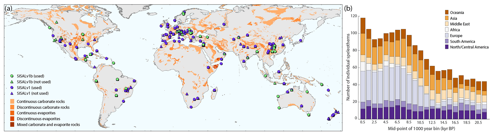
https://www.clim-past.net/15/1557/2019/cp-15-1557-2019-f01

Figure 1Spatio-temporal distribution of SISALv1b database. (a) Spatial distribution of speleothem records. Filled circles are sites used in this study (SISALv1 in blue; SISALv1b in green). Triangles are SISAL sites that do not pass the screening described in Sect. 2.3 and/or do not cover the time periods used here (modern, MH and LGM). The background carbonate lithology is that of the World Karst Aquifer Mapping (WOKAM) project (Chen et al., 2017). (b) Temporal distribution of speleothem records according to regions. The non-overlapping bins span 1000 years and start in 1950 CE. Regions have been defined as follows: Oceania ( $- 60^{\circ} < lat < 0^{\circ}$ ; $90^{\circ} < long < 180^{\circ}$ ); Asia ( $0^{\circ} < lat < 60^{\circ}$ ; $60^{\circ} < long < 130^{\circ}$ ); Middle East ( $7.6^{\circ} < lat < 50^{\circ}$ ; $26^{\circ} < long < 59^{\circ}$ ); Africa ( $- 45^{\circ} < lat < 36.1^{\circ}$ ; $- 30^{\circ} < long < 60^{\circ}$ ; with records in the Middle East region removed); Europe ( $36.7^{\circ} < lat < 75^{\circ}$ ; $- 30^{\circ} < long < 30^{\circ}$ ; plus Gibraltar and Siberian sites); South America ( $- 60^{\circ} < lat < 8^{\circ}$ ; $- 150^{\circ} < long < - 30^{\circ}$ ); North and Central America ( $8.1^{\circ} < lat < 60^{\circ}$ ; $- 150^{\circ} < long < - 50^{\circ}$ ).

The global occurrence of speleothems through time approximates an exponential distribution (Fig. 2a). Anomalously high numbers of speleothems are found in the last 12 kyr, between 128 and 112 kyr BP and during interglacials MIS 1 and 5e (and the early glacial MIS 5d). There are fewer speleothems than expected between 73 and 63 kyr BP and during MIS 2 (Fig. 2b). These deviations could arise from sampling biases, but it is unlikely that such biases would lead to differences between the tropics and temperate regions. Differences between curves constructed for both tropical and temperate regions (Fig. 2c) suggest that, at least for the last 130 ka, deviations from expected stalagmite growth in the extra-tropics correspond to variability on glacial and interglacial scales. Thus, the speleothem data indicate similar climatic sensitivity, even at a global level, to that demonstrated for sub-continental and regional scales by earlier authors, despite their use of much smaller numbers and far less precise age data than in the SISAL dataset.

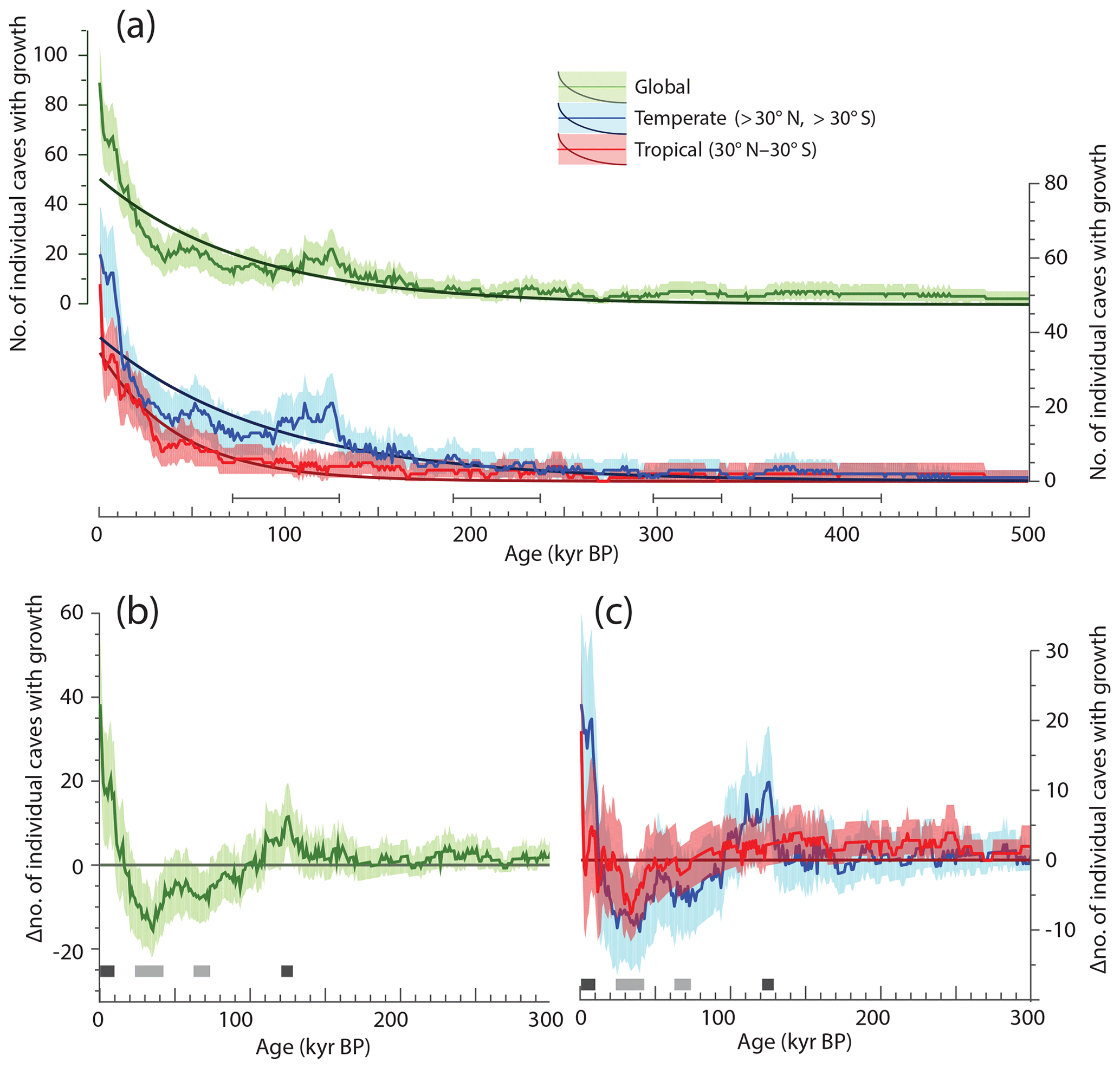
https://www.clim-past.net/15/1557/2019/cp-15-1557-2019-f02

Figure 2Distribution of the number of single caves with speleothem growth through time. (a) Number of single caves with growth over the last 500 000 yr BP (where present is 1950 CE) in 1000-year bins (solid line), bootstrapped estimate of uncertainty (shading between 5 % and 95 % percentiles) and fitted exponential distribution (darker solid line). Horizontal bars denote previous interglacials. (b, c) Same as (a) but with the fitted exponential distribution subtracted to highlight anomalies from the expected number of caves over the last 300 kyr BP. Horizontal bars indicate periods with significantly greater (dark grey) or fewer (light grey) numbers of caves with speleothem growth than expected. Green indicates the full global dataset; blue and red indicate temperate and tropical subdivisions respectively.

Download

3.2 How well do the speleothem records represent modern δ¹⁸O in precipitation?

The first-order spatial patterns shown by the SISAL speleothem records during the modern period (1960–2017; n=87) are in overall agreement with the OIPC dataset of interpolated wδ¹⁸O_p (R²=0.76), with more negative values at higher latitudes and in more continental climates (Fig. 3a). The fact that the speleothem records reflect the δ¹⁸O patterns in modern precipitation confirms at a global scale the findings of McDermott et al. (2011) for the continental scale in Europe. There are no systematic biases between OIPC and SISAL data at different latitudes (Fig. 3b). However, low latitude sites tend to show more positive δ¹⁸O values than simulated wδ¹⁸O_p, whereas sites from middle to high latitudes tend to be more negative (Fig. 3c, d). The discrepancies between the SISAL data and the observations or simulations may be due to cave-specific factors (such as a preferred seasonality of recharge, e.g. Bar-Matthews et al., 1996, or non-equilibrium fractionation processes during speleothem deposition, e.g. Ersek et al., 2018), by complex soil–atmosphere interactions affecting evapotranspiration (e.g. Denniston et al., 1999) and thus the isotopic signal of the effective recharge (Baker et al., 2019), or uncertainties in the isotope fractionation factors with respect to temperature (Fig. S1 in the Supplement) amongst others (e.g. Hartmann and Baker, 2017). However, the overall level of agreement suggests that the SISAL data provide a good representation of the impacts of modern hydroclimatic processes.

https://www.clim-past.net/15/1557/2019/cp-15-1557-2019-f03

Figure 3Comparison of SISAL data with observational and simulated $w {δ^{18} O}_{p}$ for the modern period. (a) Comparison between SISAL δ¹⁸O averages (‰; V-SMOW) for the period 1960–2017 CE with OIPC data (‰; V-SMOW). (b) Scatterplot of SISAL modern δ¹⁸O averages as in (a) versus wδ¹⁸O_p extracted from OIPC (i.e. background map in a) at the location of each cave site. (c) Same as (a) with simulated $w {δ^{18} O}_{p}$ data for the period 1958–2013 in the background. (d) Scatterplot of SISAL modern δ¹⁸O as in (c) versus the simulated $w {δ^{18} O}_{p}$ for the period 1958–2013 CE. Dashed lines in (b) and (d) represent the 1:1 line. All SISAL isotope data have been converted to their drip-water equivalent, following the approach described in Sect. 3.2. Mean annual air surface temperature from CRU-TS4.01 (Harris et al., 2014) and mean annual simulated ECHAM5-wiso air surface temperature were used as surrogates for cave temperatures in the OIPC and ECHAM5-wiso comparison, respectively. See Sect. 2.3 for details on data extraction and conversion.

Comparison of the SISAL records with δ¹⁸O_p weighted according to the potential recharge amount or with δ¹⁸O_sw weighted to the moisture amount does not significantly improve the data–model comparison (Fig. S2). The best relationship is obtained with soil water δ¹⁸O weighted according to soil moisture amount (wδ¹⁸O_sw; R²=0.76). However, smoothing the simulated wδ¹⁸O records on a sample-to-sample basis to account for multi-year transit times in the karst environment produces a slightly better geographic agreement with the SISAL records (Fig. S3). Accounting for differences between the model grid cell and cave elevations does not yield any overall improvement in the global correlations.

Simulated inter-annual variability is less than that shown in the GNIP data (Fig. 4). Although there are missing values for the GNIP station data, we have also removed these intervals from the simulations, so incomplete sampling is unlikely to explain the difference between the observed and simulated inter-annual variability. Our results are consistent with the general tendency of climate models to underestimate the sensitivity of extreme precipitation to temperature variability or trends (Flato et al., 2014). ECHAM5 is known to underestimate inter-annual variability in regions where precipitation is dominantly convective (i.e. the tropics), as well as in summer in extra-tropical regions (e.g. in southern Europe) because convective precipitation operates on small spatial scales and has a large random component, even for a given large-scale atmospheric state (Eden et al., 2012). The inter-annual variability of the modern speleothem records is lower than both the simulated and the GNIP data, reflecting the impact of karst and in-cave processes that effectively act as a low-pass filter on the signal recorded during speleothem growth (Baker et al., 2013). Thus, smoothing the simulated δ¹⁸O_p signal produces a better match to the SISAL records: application of a smoothing window of > 6 yr to simulated wδ¹⁸O_p produces a good match (95 % confidence) with the inter-annual variability shown by the speleothems (Fig. 4). This result indicates that global data–model comparisons using speleothem records should focus on quasi-decadal or longer timescales. However, the temporal smoothing caused by karst processes varies from site to site; where transmission from the surface to the cave can be shown to be rapid, individual speleothems may preserve annual or even sub-annual signals.

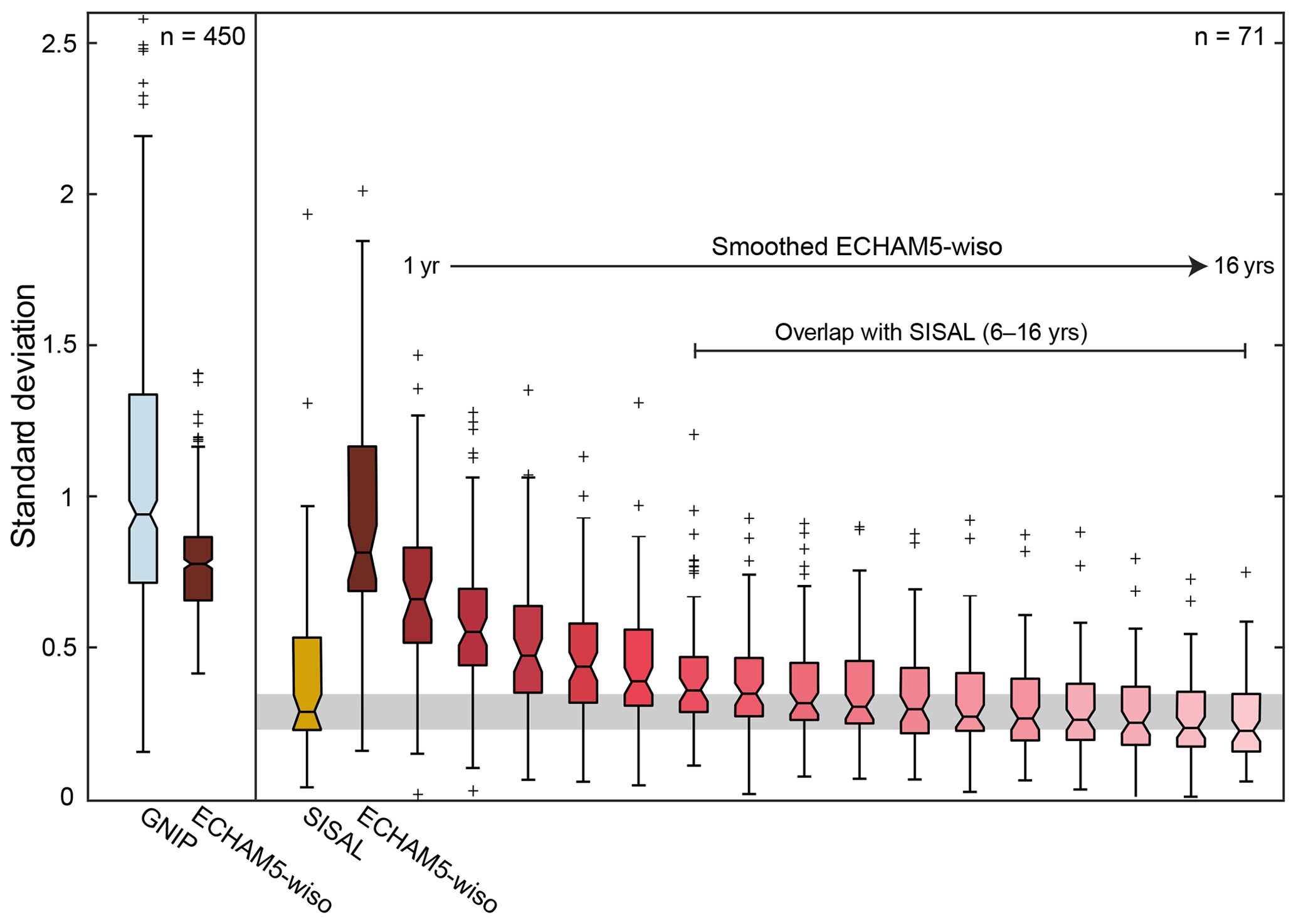
https://www.clim-past.net/15/1557/2019/cp-15-1557-2019-f04

Figure 4Modern global inter-annual δ¹⁸O variability. Box plots show the variability of the standard deviation of global annual wδ¹⁸O using (a) GNIP stations with enough months of data to account for > 80 % of the annual precipitation and at least 5 years of data (n=450) and ECHAM5-wiso data extracted at the location of each GNIP station for the years when these data are available; (b) SISAL records with at least 5 isotope samples for the period 1958–2013 and simulated wδ¹⁸O_p extracted at each cave location for the same years for which speleothem data are available. Boxplots in shades of red are constructed after smoothing the simulated wδ¹⁸O_p data for 1 to 16 years. On each box, the central mark indicates the median (q₂; 50th percentile) and the bottom and top edges of the box indicate the 25th (q₁) and 75th (q₃) percentiles, respectively. Outliers (black crosses) are locations with standard deviations greater than $q_{3} + 1.5 \times$ (q₃−q₁) or less than $q_{1} - 1.5 \times$ (q₃−q₁). This corresponds to approximately ±2.7σ or 99.3 % coverage if the data are normally distributed. If the notches in the box plots do not overlap, you can conclude, with 95 % confidence, that the true medians do differ. The grey horizontal band corresponds to the notch in SISAL for easy comparison. SISAL data were converted to their drip-water δ¹⁸O equivalent as described in Sect. 2.3.

Download

3.3 Anomaly-mode time-slice comparisons

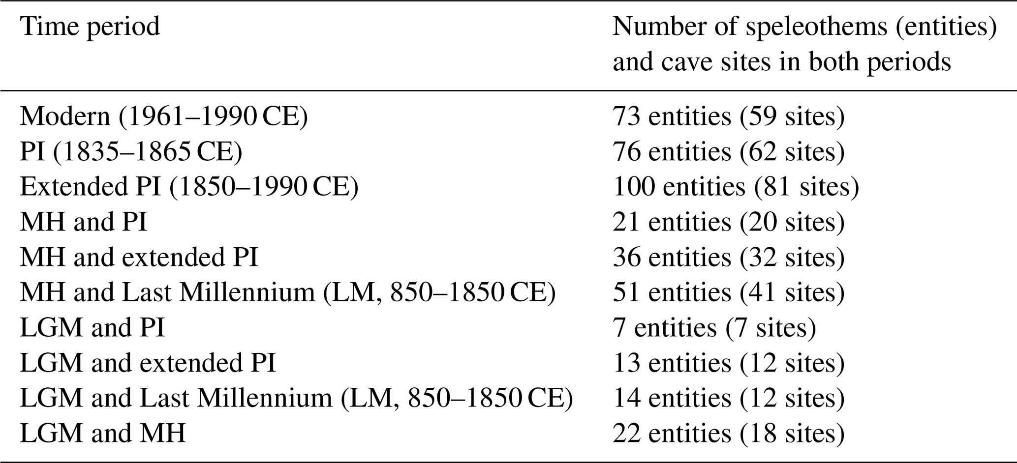
The selection of a modern or pre-industrial base period is a first step in reconstructing speleothem δ¹⁸O anomalies for comparisons with simulated changes in specific model experiments. There are 76 speleothem records from 62 sites that cover the pre-industrial interval (PI) 1850±15 CE, commonly used as a reference in model experiments. However, using this short interval as the base period for comparisons with MH or LGM simulations would result in the reconstruction of anomalies for only 21 records for the MH and only 7 records for the LGM – which are the number of speleothem records with isotope samples in both the base period and either the MH or LGM (Table 2). There is no significant difference in the mean δ¹⁸O values for this pre-industrial period and the modern δ¹⁸O values (R²=0.96; Fig. S4). Using an extended modern baseline (1850–1990 CE) increases the data uncertainties by only ±0.5 ‰ but raises the number of MH records for which MH–modern anomalies can be calculated to 36 entities from 32 sites around the world. There is also an improvement in the number of LGM sites for which it is possible to calculate anomalies, from 7 to 13 entities at 12 sites. Although longer base periods have been used for data–model comparisons, for example the last 1000 years (e.g. Werner et al., 2016), this would increase the uncertainties in the observations without substantially increasing the number of records for which it would be possible to calculate anomalies, particularly for the LGM (Table 2). We, therefore, recommend the use of the interval 1850–1990 CE as the baseline for calculation of δ¹⁸O anomalies from the speleothem records.

Table 2Number of SISALv1b speleothem records available for key time periods. Mid-Holocene (MH): 6±0.5 kyr BP; Last Glacial Maximum (LGM): 21±1 kyr BP. The term “kyr BP” refers to thousand years before present, where present is 1950 CE.

Download Print Version | Download XLSX

A relatively good agreement exists between the sign of the simulated and observed δ¹⁸O changes at the MH and LGM: 94 % of the MH entities and 84 % of the LGM entities show changes in the same direction after allowing for an uncertainty of ±0.5 ‰ (Fig. 5a, b). However, the magnitude of the changes is larger in the SISAL records than the simulations. The MH–modern speleothem anomalies range from −3.60 ‰ to 1.29 ‰ (mean ± SD: $- 0.50 \pm 1.01$ ‰), but the simulated anomalies only range from −0.49 ‰ to 0.28 ‰ (mean ± SD: 0.00±0.32 ‰). Observed anomalies are 4–20 times larger than simulated anomalies in the Asian monsoon region, and in individual sites in North and South America and Uzbekistan (Fig. 5a). The data–model mismatch is smallest in Europe, with a mean data–model offset of $- 0.13 \pm 0.42$ ‰ (n=9 entities from 7 sites). A two-tailed Student t test shows that most of the simulated MH values are not significantly different from those of the present (at 95 % confidence). This may reflect the fact that the midHolocene simulation was only run for 10 years but is also consistent with previous studies which show that climate models substantially underestimate the magnitude of MH changes (Harrison et al., 2014), particularly in monsoon regions (e.g. Perez-Sanz et al., 2014).

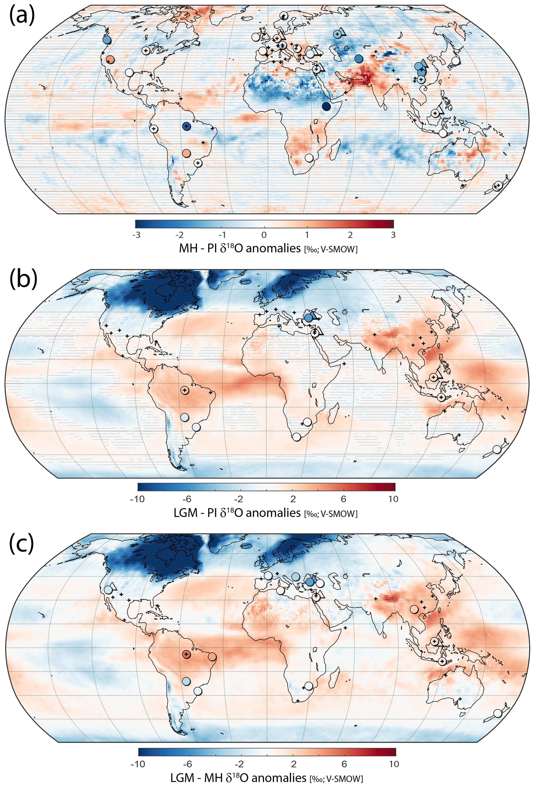
https://www.clim-past.net/15/1557/2019/cp-15-1557-2019-f05

Figure 5ECHAM5-wiso weighted δ¹⁸O_p anomalies (‰; V-SMOW; background map) and SISAL isotope anomalies (‰; V-SMOW; filled circles) for three time slices: (a) MH-PI (SISAL records, n=36), (b) LGM-PI (SISAL records, n=13) and (c) LGM–MH (SISAL records, n=22). For easy visualization, when there are two speleothem records from the same cave site, one has been shifted 2^∘ towards the north and the east (shown here as triangles). Note the different colour bar axis in the colour bar of (a) compared to (b) and (c). Two-tailed student t test has been applied to calculate the significance of the ECHAM5-wiso anomalies in (a) and (b) at a 95 % confidence. No significance has been calculated for (c), which compares two different simulations with their corresponding control periods. SISAL anomalies calculated with respect to 1850–1990 CE. Small black crosses indicate SISAL entities that do not have a modern equivalent. SISAL data have been converted to their drip water equivalent prior to calculating the anomalies as described in Sect. 2.3.

The simulated changes in δ¹⁸O at the LGM are much larger than those simulated for the MH and are significant (at 95 % confidence) over much of the globe. There is no regionally coherent pattern in the observed LGM anomalies because of the limited number of speleothems that grew continuously from the LGM to the present. However, the sign of the observed changes is coherent with the simulated change in δ¹⁸O for 11 of the 13 records (Fig. 5b). The magnitude of the LGM anomalies differs by less than 1 ‰ between model and data in two-thirds of the locations. A strong offset is found in the two records from Sofular Cave, which are ca. 5.5 ‰ more negative than the simulated δ¹⁸O. This offset may be related to the glacial changes in the Black Sea region, which are not well represented in the lgm simulation. Thus, although overall the comparison with the speleothem records suggests that the simulated changes in hydroclimate are reasonable, the simulated changes in the Middle East differ from observations.

An alternative approach to examine the realism of simulated changes is to compare the LGM and MH periods directly, which improves the number of records for which anomalies can be calculated (Fig. 5c; n=22). However, the pattern of change is similar to the LGM–modern anomalies. The simulated and observed direction of change is coherent at 86 % of the locations with an offset smaller than 1 ‰ occurring in 12 sites, and again the largest discrepancy is Sofular Cave. Thus, in this particular example, a direct comparison of the LGM–MH anomalies does not provide additional insight to the comparison of LGM–modern anomalies. Nevertheless, such an approach might be useful for other time periods (e.g. comparison of early versus mid-Holocene) when there are likely to be many more speleothem records available.

Age uncertainties inherent to the speleothem samples representing the LGM could partially explain the LGM data–model mismatches. A global assessment of the impact of time-window width on the MH and LGM anomalies shows that reducing the window width from ±500 to ±200 years in the MH has little impact on the average values (Fig. S5) but reduces the inter-sample variability and produces a better match to the simulated anomalies. A similar analysis for the LGM (Fig. S6) suggests that a window width of ±500 years (rather than ±1000 years) would be the most appropriate choice for comparisons of this interval. The number of SISAL sites available for such comparisons is not affected. However, analyses of the relative error of the isotope anomalies calculated at individual sites for different LGM window widths (Fig. 6) show a clear increase in all relative error components as window size decreases for BT-2 (Botuverá cave; Fig. 6a; Cruz et al., 2005) but no clear changes in the relative error terms for SSC01 (Gunung-buda cave; Fig. 6b; Partin et al., 2007). These results suggest that, with an LGM window width of ±1000 years, the relative contribution of age uncertainty to the anomaly uncertainty is small (Fig. 6). Thus, although it is clear that it would be useful to propagate age uncertainties for individual sites, changing the conventional definitions of the MH and LGM time slices in deriving speleothem anomalies does not seem warranted at this stage.

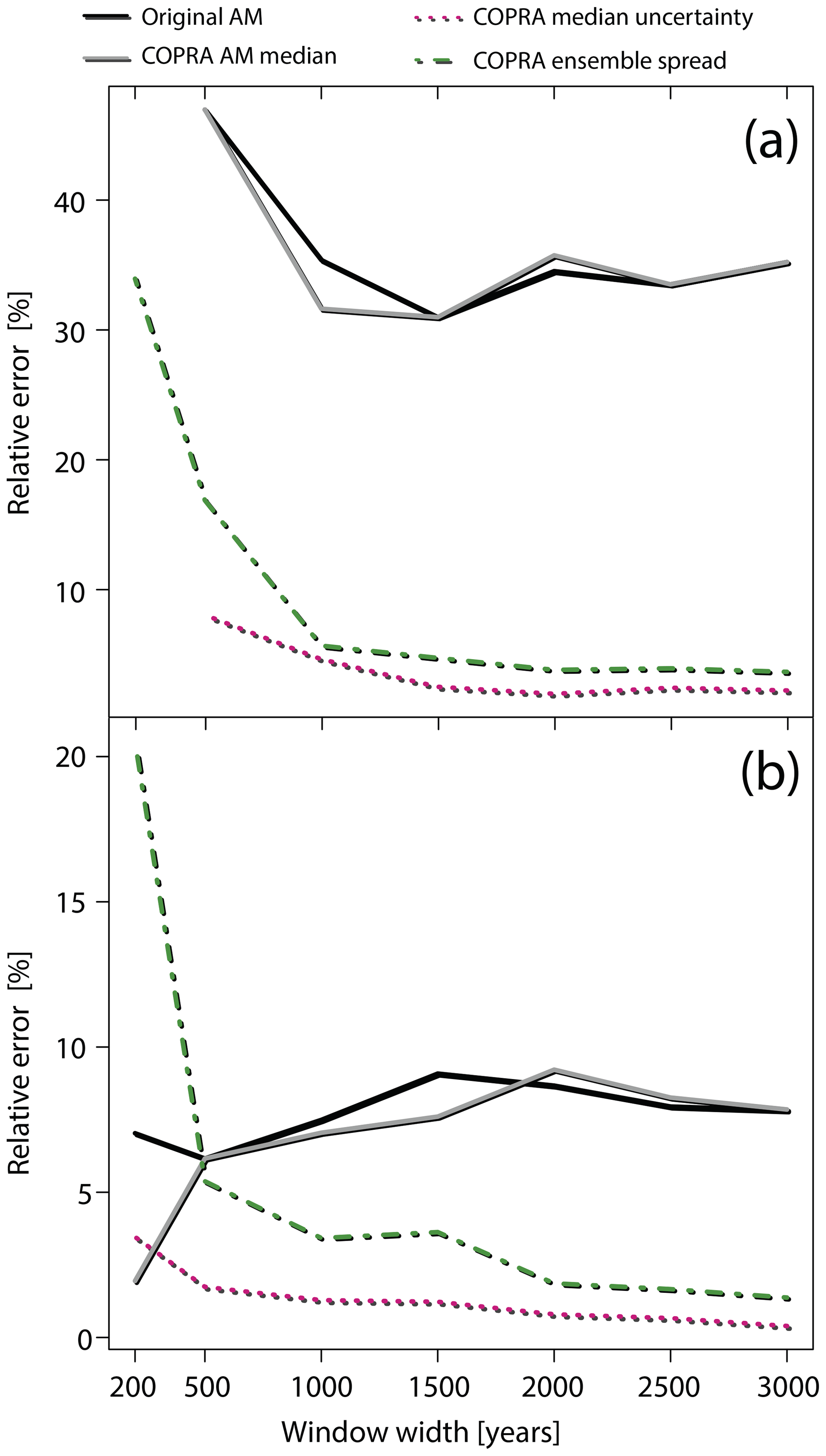
https://www.clim-past.net/15/1557/2019/cp-15-1557-2019-f06

Figure 6LGM period definitions and their impact on SISAL δ¹⁸O mean estimate uncertainty. The impact of the window definition and age uncertainty is explored for two entities: (a) entity BT-2 from Botuverá cave (Cruz et al., 2005) and (b) entity SSC01 from Gunung-buda cave (Partin et al., 2007). The relative error is defined as 2 standard deviation for the original age model and the COPRA median; and the upper minus lower 95 % quantiles for the COPRA median uncertainty as well as the COPRA ensemble spread of standard deviations. Black solid lines give the relative error of the mean isotope estimate for the LGM for the original age model and grey solid lines give the estimate based on the COPRA median age model. The pink dotted line shows the uncertainty of the COPRA median estimate, and the green dashed line the average relative error estimate across the 1000-member COPRA ensemble. For both speleothems, relatively stable error estimates are found for window sizes larger than ±750 years, whereas the relative error increases towards smaller window sizes.

Download

3.4 Analysis of spatial gradients

The number of sites available in SISALv1b means that quantitative data–model comparisons using the traditional anomaly approach are limited in scope. Approaches based on comparing trends in absolute δ¹⁸O values could provide a way of increasing the number of observations and an alternative way to evaluate the simulations. Comparison of trends places less weight on anomalous sites and allows large-scale systematic similarities and dissimilarities between model and observations to be revealed. We illustrate this approach using spatial gradients across Asia and across Europe and showing how they differ between the modern, MH and LGM periods, although such an approach could also be used for temporal trends.

The first-order spatial gradient in observed δ¹⁸O during the modern period is broadly captured by the model in both examples (Figs. 7, 8), with the largest offsets found mainly for high-altitude sites. There is a fundamental change in the latitudinal gradient across Asia during the MH (Fig. 7). In this period, the gradient observed in the data is clearly not reproduced by the model, which systematically simulates higher wδ¹⁸O_p values between 20 and 35^∘ N, suggesting that the model underestimates the insolation-driven intensification of the hydrological cycle in monsoon regions during this period. The limited number of speleothem records available between 25 and 35^∘ N for the LGM agree with the simulated δ¹⁸O gradient. The longitudinal gradient across Europe (Fig. 8) does not change substantially in the MH compared to modern times. However, the model simulates wδ¹⁸O_p values ∼2 ‰ lower than observed in low-altitude sites in south central Europe between 0 and 15^∘ E during the MH. This suggests that the model may be underestimating the role of atmospheric circulation (i.e. weaker westerlies) during this period, an aspect of the climate system that models have difficulty simulating (Mauri et al., 2014). The large latitudinal variability of simulated values eastwards of ∼5^∘ E during the LGM is consistent with a larger spread in the observations, despite the limited number of data available. These examples show the potential to use trends in absolute values for model evaluation and diagnosis.

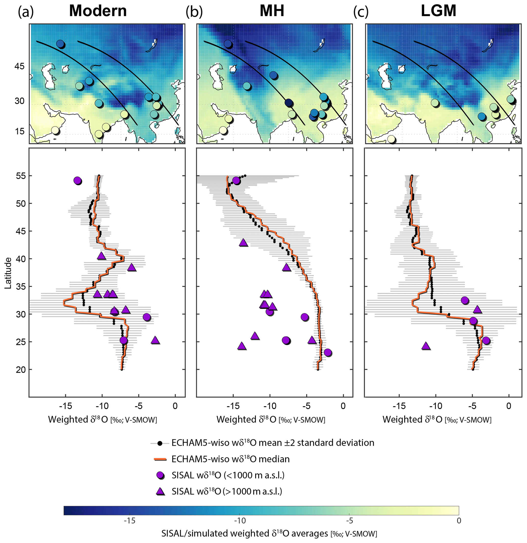
https://www.clim-past.net/15/1557/2019/cp-15-1557-2019-f07

Figure 7Latitudinal isotopic transect for Asia during the (a) modern (1958–2013 CE), (b) Mid-Holocene (MH; 6±0.5 kyr BP) and (c) Last Glacial Maximum (LGM; 20±1 kyr BP) periods. Background maps at the top of each panel show the simulated $w {δ^{18} O}_{p}$ from ECHAM5-wiso. Bottom plots in each panel show the simulated $w {δ^{18} O}_{p}$ data extracted for each transect: black circles and grey whiskers are mean ±2 standard deviation of the data extracted along longitudinal sections in between the two great circle lines shown in solid black lines in the top maps. The red line is the median of the extracted data. All data were extracted at steps of 1.12^∘ to coincide with the average model grid size. These bottom panels also show SISAL δ¹⁸O: circles for low-elevation sites, < 1000 m a.s.l.; triangles for high-elevation sites, > 1000 m a.s.l.

https://www.clim-past.net/15/1557/2019/cp-15-1557-2019-f08

Figure 8Longitudinal isotopic transect for Europe during the (a) modern (1958–2013 CE), (b) Mid-Holocene (MH; 6±0.5 kyr BP) and (c) Last Glacial Maximum (LGM; 20±1 kyr BP) periods. Details as in caption of Fig. 7.

4 Protocol for data–model comparison using speleothem data

Our analyses illustrate a number of possible approaches for using speleothem isotope data for model evaluation. The discontinuous nature of most speleothem records means that the number of sites available for conventional anomaly-mode comparisons is potentially limited. To some extent this is mitigated by the fact that differences between the modern and pre-industrial isotope values are small, permitting the calculation of anomalies using a longer baseline interval (1850–1990 CE). The use of smaller intervals of time in calculating MH or LGM anomalies (Figs. S5 and 6) does not have a significant impact either on the mean values or the number of records provided the interval is >±300 yr for the MH and >±500 yr for the LGM. Although the use of shorter intervals is possible, we recommend using the conventional definitions of each time slice to facilitate comparison with other benchmark datasets. Although patterns in the isotope anomalies can provide a qualitative assessment of model performance, site-specific factors could lead to large differences from the simulations at individual locations. Improved spatial coverage would allow such sites to be identified and screened out before making quantitative comparisons of observed and simulated anomalies. Although there are only a limited number of records that cover both the modern baseline period and the MH (or the modern baseline period and the LGM), there are many more records that provide information about one or other of these periods. The examination of spatial gradients in absolute δ¹⁸O provides one way of exploiting this larger data coverage. Even when an offset between the observed and simulated δ¹⁸O exists, comparing the trends along such gradients is possible. Thus, both absolute values and anomalies of the isotope data for data–model comparison are useful.

Screening of published speleothem isotope data is essential to produce meaningful data–model comparisons. The SISAL database facilitates screening for mineralogy, which has a substantial effect on isotope values because of differences in water-carbonate fractionation factors for aragonite or calcite that are more pronounced at lower temperatures (Fig. S1).

Based on the limited number of records available at the LGM, speleothem age uncertainties have only a limited impact on mean isotope values, and propagation of such uncertainties as well as any model uncertainties would nevertheless substantially improve the robustness of data–model comparisons.

Based on our analyses, we therefore recommend that model evaluation using speleothem records should do the following:

filter speleothem records with respect to their mineralogy and use the appropriate equilibrium fractionation factor: Tremaine et al. (2011) for converting isotope data from either calcite or aragonite-corrected-to-calcite samples to their drip water equivalent, and Grossman and Ku (1986) as reformulated by Lachniet (2015) for converting isotope data from aragonite samples;
use the interval between 1850 and 1990 as the reference period for speleothem isotope records;
use speleothem isotope data averaged for the intervals 6000±500 yr (21 000±1000 yr) for comparability with other MH (LGM) palaeoclimate benchmark datasets;
use speleothem isotope data averaged for the interval 6000±200 yr or 21 000±500 yr for best approximation of midHolocene and lgm experiments;
use absolute values only to assess data–model first order spatial patterns;
focus on multi-decadal to millennial timescales if using transient simulations for data–model comparisons.

5 Conclusions

Speleothem records show the same first-order spatial patterns as are available in the Global Network of Isotopes in Precipitation (GNIP) data and are therefore a good reflection of the δ¹⁸O patterns in modern precipitation. This observation suggests that stalagmites are a rich source of information for model evaluation. However, the inter-annual variability in the modern speleothem records is considerably reduced compared to the simulations, which in turn show less inter-annual variability than the GNIP observations. The low variability shown by the SISAL records – most likely from the low-pass filter effectively applied to the speleothem record by the karst system – precludes the use of this database for global studies focused on timescales shorter than quasi-decadal.

Using the traditional anomaly approach to data–model comparisons, there is consistency between the sign of observed and simulated changes in both the MH and the LGM. However, the ECHAM5-wiso model underestimates the changes in δ¹⁸O between time periods compared to the speleothem records (i.e. the amplitude of modelled δ¹⁸O changes is lower). Thus, these kinds of comparisons should only focus on the large-scale spatial patterns. Based on the available SISAL data, the use of smaller time windows than the conventional definitions for each time slice does not have a strong impact on the mean values and could be used to reduce the uncertainties associated with the palaeodata. However, this would preclude comparisons with existing benchmark datasets that use the conventional windows for the MH and LGM time slices.

Only a limited number of speleothem records are continuous over long periods of time and the need to convert these to anomalies with respect to modern times is a drawback. The limited number of records covering the LGM make the comparisons for this period particularly challenging. Nevertheless, continued expansion of the SISAL database will increase its usefulness for model evaluation in future. Furthermore, we have shown that alternative approaches using absolute values could help examine spatial trends and diagnose systematic offsets.

Mismatches between simulations and observations can reflect the issues with the experimental design, problems with the model or uncertainties in the observations (Harrison et al., 2015). The failure to include changes in atmospheric dust loading, for example, has been put forward as an explanation of data–model mismatches in both the MH and the LGM (e.g. Hopcroft et al., 2015; Messori et al., 2019). Missing processes and feedbacks, such as climate-induced vegetation or land-surface changes, could also contribute to mismatches (e.g. Yoshimori et al., 2009; Swann et al., 2014). Uncertainties caused by the specific structure of the model or assigned model parameter values could also contribute to data–model mismatches (Qian et al., 2016). Ultimately, there needs to be an assessment of the contribution of all these factors to data–model mismatches, but here we have only focused on potential uncertainties associated with the speleothem data. Our initial analyses suggest age uncertainty contributes little to the uncertainties in the estimates of LGM speleothem isotope values. However, it is still important to propagate dating uncertainties for data–model comparison. Site-specific controls may have a much larger effect on the δ¹⁸O record recorded by individual speleothems and thus may contribute significantly to uncertainties in local or regional signals. We have not screened for regionally anomalous records that could be influencing the results of our analyses, but this should certainly be done. Despite these challenges, SISAL appears to be an extremely useful tool for describing past patterns of variability, highlighting its potential for evaluating CMIP6-PMIP4 experiments.

Comparisons with speleothem data can be seen as a complement to model evaluation using other types of palaeoenvironmental data and palaeoclimatic reconstructions (see for example MARGO Project Members, 2009; Harrison et al., 2014). They are particularly useful because they provide insights into how well state-of-the-art models reproduce the hydrological cycle and atmospheric circulation patterns. The ability to reproduce past observations provides additional confidence in the ability of climate models to simulate large climate changes, such as those expected by the end of the 21st century (Braconnot et al., 2012; Schmidt et al., 2014). However, mismatches between model simulations and palaeo-observations are also useful because they can help to pinpoint issues that may need to be addressed in developing improved models or in better experimental protocols (Kageyama et al., 2018), providing that these mismatches do not arise because of misunderstanding or misinterpretation of the observations themselves. By providing a protocol for using speleothem data for data–model comparisons that accounts for uncertainties in the observations, we anticipate that at least such causes of data–model mismatches will be minimized.

Data availability

The SISAL (Speleothem Isotopes Synthesis and AnaLysis Working Group) database version 1b is publicly available through the University of Reading repository at http://doi.org/10.17864/1947.189 (Atsawawaranunt et al., 2019) and through the NOAA's National Centers for Environmental Information (NCEI) at https://www.ncdc.noaa.gov/paleo-search/study/24070. The ECHAM5-wiso model output is available from https://doi.org/10.1594/PANGAEA.902347 (Werner, 2019). The OIPC mean annual precipitation δ¹⁸O data are available from the Water Isotopes Database at http://wateriso.utah.edu/waterisotopes/pages/data_access/ArcGrids.html (Bowen and Revenaugh, 2003; IAEA/WMO, 2015; Bowen, 2018). The Global Network of Isotopes in Precipitation (GNIP; IAEA/WMO, 2018) data from the International Atomic Energy Agency (IAEA) and the World Meteorological Organization (WMO) are available at https://nucleus.iaea.org/wiser.

Supplement

The supplement related to this article is available online at: https://doi.org/10.5194/cp-15-1557-2019-supplement.

Team list

SISAL working group members who coordinated data gathering for the SISAL database are listed here in alphabetical order: Syed Masood Ahmad (Department of Geography, Faculty of Natural Sciences, Jamia Millia Islamia, New Delhi 110025, India), Yassine Ait Brahim (Institute of Global Environmental Change, Xi'an Jiaotong University, Xi'an, Shaanxi, China), Sahar Amirnezhad Mozhdehi (School of Earth Sciences, University College Dublin, Belfield, Dublin 4, Ireland), Monica Arienzo (Division of Hydrologic Sciences, Desert Research Institute, 2215 Raggio Parkway, 89512 Reno, NV, USA), Kamolphat Atsawawaranunt (School of Archaeology, Geography & Environmental Sciences, Reading University, Whiteknights, Reading, RG6 6AH, UK), Andy Baker (School of Biological, Earth and Environmental Sciences, University of New South Wales, Kensington 2052, Australia), Kerstin Braun (Institute of Human Origins, Arizona State University, P.O. Box 874101, 85287 Tempe, Arizona, USA), Sebastian Breitenbach (Sediment & Isotope Geology, Institute of Geology, Mineralogy & Geophysics, Ruhr-Universität Bochum, Universitätsstr. 150, IA E5-179, 44801 Bochum, Germany), Yuval Burstyn (Geological Survey of Israel, 32 Yesha'yahu Leibowitz, 9371234, Jerusalem, Israel; Institute of Earth Sciences, Hebrew University of Jerusalem, Edmond J. Safra campus, Givat Ram, 91904 Jerusalem, Israel), Sakonvan Chawchai (MESA Research unit, Department of Geology, Faculty of Sciences, Chulalongkorn University, 254 Phayathai Rd, Pathum Wan, 10330 Bangkok, Thailand), Andrea Columbu (Department of Biological, Geological and Environmental Sciences, Via Zamboni 67, 40126, Bologna, Italy), Michael Deininger (Institute of Geosciences, Johannes Gutenberg University Mainz, Johann-Joachim-Becher-Weg 21, 55128 Mainz, Germany), Attila Demény (Institute for Geological and Geochemical Research, Research Centre for Astronomy and Earth Sciences, Hungarian Academy of Sciences, Budaörsi út 45, 1112 Budapest, Hungary), Bronwyn Dixon (School of Archaeology, Geography & Environmental Sciences, Reading University, Whiteknights, Reading, RG6 6AH, UK; School of Geography, University of Melbourne, Melbourne, 3010, Australia), István Gábor Hatvani (Institute for Geological and Geochemical Research, Research Centre for Astronomy and Earth Sciences, Hungarian Academy of Sciences, Budaörsi út 45, 1112 Budapest, Hungary), Jun Hu (Department of Earth Sciences, University of Southern California, 3651 Trousdale Parkway, 90089 Los Angeles, California, USA), Nikita Kaushal (Department of Earth Sciences, University of Oxford, South Parks Road, Oxford, OX1 3AN, UK), Zoltán Kern (Institute for Geological and Geochemical Research, Research Centre for Astronomy and Earth Sciences, Hungarian Academy of Sciences, Budaörsi út 45, 1112 Budapest, Hungary), Inga Labuhn (Institute of Geography, University of Bremen, Celsiusstr. 2, 28359 Bremen, Germany), Matthew S. Lachniet (Dept. of Geoscience, University of Nevada Las Vegas, P.O. Box 4022, 89154 Las Vegas, NV, USA), Franziska A. Lechleitner (Department of Earth Sciences, University of Oxford, South Parks Road, OX1 3AN Oxford, UK), Andrew Lorrey (National Institute of Water & Atmospheric Research, Climate Atmosphere and Hazards Centre, 41 Market Place, Viaduct Precinct, Auckland, New Zealand), Monika Markowska (University of Tübingen, Hölderlinstr. 12, 72074 Tübingen, Germany), Carole Nehme (IDEES UMR 6266 CNRS, Geography department, University of Rouen Normandie, Mont Saint Aignan, France), Valdir F. Novello (Instituto de Geociências, Universidade de São Paulo, São Paulo, Brazil), Jessica Oster (Department of Earth and Environmental Sciences, Vanderbilt University, Nashville, TN, 37206, USA), Carlos Pérez-Mejías (Department of Geoenvironmental Processes and Global Change, Pyrenean Institute of Ecology (IPE-CSIC), Avda. Montañana 1005, 50059 Zaragoza, Spain, now at: Institute of Global Environmental Change, Xi’an Jiaotong University, Xi’an, Shaanxi, China), Robyn Pickering (Department of Geological Sciences, South Africa and Human Evolution Research Institute, South Africa), Natasha Sekhon (Department of Geological Sciences, Jackson School of Geosciences, University of Texas, Austin, TX, 78712, USA), Xianfeng Wang (Earth Observatory of Singapore, Nanyang Technological University, 636798, Singapore), Sophie Warken (Institute of Environmental Physics, Ruprecht-Karls-Universität Heidelberg, Im Neuenheimer Feld 229, 69120 Heidelberg, Germany).

SISAL working members who submitted data to the SISAL database are listed here in alphabetical order: Tim Atkinson (Departments of Earth Sciences & Geography, University College London, WC1E 6BT, UK), Avner Ayalon (Geological Survey of Israel, 32 Yesha'yahu Leibowitz, 9371234 , Jerusalem), James Baldini (Department of Earth Sciences, Durham University, DH1 3LE, UK), Miryam Bar-Matthews (Geological Survey of Israel, 32 Yesha'yahu Leibowitz, , 9371234 , Jerusalem), Juan Pablo Bernal (Centro de Geociencias, Universidad Nacional Autónoma de México, Campus UNAM Juriquilla, Querétaro 76230, Querétaro, Mexico), Ronny Boch (Graz University of Technology, Institute of Applied Geosciences, Rechbauerstrasse 12, 8010 Graz, Austria), Andrea Borsato (School of Environmental and Life Science, University of Newcastle, 2308 NSW, Australia), Meighan Boyd (Department of Earth Sciences, Royal Holloway University of London, Egham, Surrey TW20 0EX, UK), Chris Brierley (Department of Geography, University College London, WC1E 6BT, UK), Yanjun Cai (State Key Lab of Loess and Quaternary Geology, Institute of Earth Environment, Chinese Academy of Sciences, Xi'an 710061, China), Stacy Carolin (Institute of Geology, University of Innsbruck, Innrain 52, 6020 Innsbruck, Austria), Hai Cheng (Institute of Global Environmental Change, Xi'an Jiaotong University, China), Silviu Constantin (Emil Racovita Institute of Speleology, str. Frumoasa 31, Bucharest, Romania), Isabelle Couchoud (EDYTEM, UMR 5204 CNRS, Université Savoie Mont Blanc, Université Grenoble Alpes, 73370 Le Bourget du Lac, France), Francisco Cruz (Instituto de Geociências, Universidade de São Paulo, São Paulo, Brazil), Rhawn Denniston (Department of Geology, Cornell College, Mount Vernon, IA, 52314, USA), Virgil Drăguşin (Emil Racovita Institute of Speleology, Str. Frumoasa 31, Bucharest, Romania), Wuhui Duan (Key Laboratory of Cenozoic Geology and Environment, Institute of Geology and Geophysics, Chinese Academy of Sciences, Beijing, 100029, China), Vasile Ersek (Department of Geography and Environmental Sciences, Northumbria University, Newcastle upon Tyne, UK), Martin Finné (Department of Archaeology and Ancient History, Uppsala University, Sweden), Dominik Fleitmann (Department of Archaeology, School of Archaeology, Geography and Environmental Science, Whiteknights, University of Reading RG6 6AB, UK), Jens Fohlmeister (Institute for Earth and Environmental Sciences, University of Potsdam, Karl-Liebknecht-Str. 24–25, 14476 Potsdam, Germany), Amy Frappier (Department of Geosciences, Skidmore College, Saratoga Springs, NY 12866, USA), Dominique Genty (Laboratoire des Science du Climat et de l'Environment, CNRS, L'Orme des Merisiers, 91191 Gif-sure-Yvette Cedex, France), Steffen Holzkämper (Department of Physical Geography, Stockholm University, 106 91 Stockholm, Sweden), Philip Hopley (Department of Earth and Planetary Sciences, Birkbeck, University of London, Malet St, London, WC1E 7HX, UK), Vanessa Johnston (Karst Research Institute, Research Centre of the Slovenian Academy of Sciences and Arts, Titov trg 2, 6230, Postojna, Slovenia), Gayatri Kathayat (Institute of Global Environmental Change, Xi'an Jiaotong University, China), Duncan Keenan-Jones (School of Historical and Philosophical Inquiry, University of Queensland, St Lucia QLD 4072, Australia), Gabriella Koltai (Institute of Geology, University of Innsbruck, Innrain 52, 6020 Innsbruck, Austria), Ting-Yong Li (Chongqing Key Laboratory of Karst Environment, School of Geographical Sciences, Southwest University, Chongqing 400715, China; Field Scientific Observation & Research Base of Karst Eco-environments at Nanchuan in Chongqing, Ministry of Nature Resources of China, Chongqing 408435, China), Mahjoor Ahmad Lone (High-Precision Mass Spectrometry and Environment Change Laboratory (HISPEC), Department of Geosciences, National Taiwan University, Taipei 10617, Taiwan, China. Research Center for Future Earth, National Taiwan University, Taipei 10617, Taiwan, China), Marc Luetscher (Swiss Institute for Speleology and Karst Studies (SISKA), Rue de la Serre 68, CH-2301 La Chaux-de-Fonds, Switzerland), Dave Mattey (Department of Earth Sciences, Royal Holloway University of London, Egham, Surrey, TW20 0EX, UK), Ana Moreno (Dpto. de Procesos Geoambientales y Cambio Global, Instituto Pirenaico de Ecología-CSIC, Zaragoza, Spain), Gina Moseley (Institute of Geology, University of Innsbruck, Innrain 52, 6020 Innsbruck, Austria), David Psomiadis (Imprint Analytics GmbH, Werner von Siemens Str. 1, A7343 Neutal, Austria), Jiaoyang Ruan (Guangdong Provincial Key Lab of Geodynamics and Geohazards, School of Earth Sciences and Engineering, Sun Yat-sen University, Guangzhou 510275, China), Denis Scholz (Institute for Geosciences, University of Mainz, Johann-Joachim-Becher-Weg 21, 55128 Mainz, Germany), Lijuan Sha (Institute of Global Environmental Change, Xi'an Jiaotong University, Xi'an, Shaanxi, China), Andrew Christopher Smith (NERC Isotope Geoscience Facility, British Geological Survey, Nottingham, UK), Nicolás Strikis (Departamento de Geoquímica, Universidade Federal Fluminense, Niterói, Brazil), Pauline Treble (ANSTO, Lucas Heights NSW, Australia), Ezgi Ünal-İmer (Department of Geological Engineering, Middle East Technical University, Ankara, Turkey), Anton Vaks (Geological Survey of Israel, 32 Yesha'yahu Leibowitz, 9371234, Jerusalem), Stef Vansteenberge (Analytical, Environmental & Geo-Chemistry, Department of Chemistry, Vrije Universiteit Brussel, Belgium), Ny Riavo G. Voarintsoa (Institute of Earth Sciences, The Hebrew University in Jerusalem, Israel), Corinne Wong (Environmental Science Institute, The University of Texas at Austin, 2275 Speedway, Austin TX 78712, USA), Barbara Wortham (Department of Earth and Planetary Science, University of California, Davis, USA), Jennifer Wurtzel (Research School of Earth Sciences, Australian National University, Canberra, ACT, Australia/ARC Centre of Excellence for Climate System Science, Australian National University, Canberra, ACT, Australia), Haiwei Zhang (Institute of Global Environmental Change, Xi'an Jiaotong University, China).

Author contributions

LCB is the coordinator of the SISAL working group. LCB and SPH designed the study. LCB and SPH wrote the first draft of the manuscript with contributions from MW, NS, KR and CVP. LCB did the analyses and created Figs. 1, 3–5, 7, 8 and S1–6. MW provided the ECHAM5-wiso model simulations and helped with model analyses. NS did the analyses on speleothem growth over time and created Fig. 2. KR did the analysis on the LGM uncertainties and created Fig. 6. All authors contributed to the last version of this paper. The authors listed in the “SISAL working group” team contributed to this study by coordinating data gathering, by database construction or with speleothem data submitted to the SISAL database. SB created the COPRA age–depth models used in this study. TA and DG contributed original unpublished data to the SISAL database. AB, BW, JB, MA, MSL, SB, TA, VJ and ZK helped edit the paper.

Competing interests

The authors declare that they have no conflict of interest.

Acknowledgements

SISAL (Speleothem Isotopes Synthesis and Analysis) is a working group of the Past Global Changes (PAGES) programme. We thank PAGES for their support for this activity. We thank the World Karst Aquifer Mapping project (WOKAM) team for providing us with the karst map presented in Fig. 1a. The authors would like to thank the following data contributors: Petra Bajo, Dominique Blamart, Russell Drysdale, Frank McDermott and Jean Riotte. Laia Comas-Bru and Sandy P. Harrison acknowledge support from the ERC-funded project GC2.0 (Global Change 2.0: Unlocking the past for a clearer future, grant no. 694481). Sandy P. Harrison also acknowledges support from the JPI-Belmont project “PAleao-Constraints on Monsoon Evolution and Dynamics (PACMEDY)” through the UK Natural Environmental Research Council (NERC). Laia Comas-Bru also acknowledges support from the Geological Survey Ireland (Short Call 2017; grant number 2017-SC-056) and the Royal Irish Academy's Charlemont Scholar award 2018. Cristina Veiga-Pires acknowledges funding from the Portuguese Science Foundation (FCT) through the CIMA research centre project UID/MAR/00350/2013. Kira Rehfeld was supported by Deutsche Forschungsgemeinschaft (DFG) grant no. RE3994/2-1.

Financial support

Financial support for SISAL activities that have lead to this research has been provided by the Past Global Changes (PAGES) programme; the European Geosciences Union (grant no. W2017/413); the Irish Centre for Research in Applied Geosciences (iCRAG); the European Association of Geochemistry (Early Career Ambassadors program 2017); the Quaternary Research Association UK; the Navarino Environmental Observatory, Stockholm University; University College Dublin (grant no. SF1428), Savillex (UK); John Cantle; Ibn Zohr University, Morocco; the University of Reading; the European Research Council (grant no. 694481); the Natural Environment Research Council (JPI-Belmont project “PAleao-Constraints on Monsoon Evolution and Dynamics (PACMEDY)”); the Geological Survey Ireland (grant no. 2017-SC-056); the Royal Irish Academy (Charlemont Scholar award 2018); the Portuguese Science Foundation (grant no. UID/MAR/00350/2013); and the Deutsche Forschungsgemeinschaft (grant no. RE3994/2-1).

Review statement

This paper was edited by Zhengtang Guo and reviewed by three anonymous referees.

References

Atkinson, T. C., Harmon, R. S., Smart, P. L., and Waltham, A. C.: Palaeoclimatic and geomorphic implications of ²³⁰Th∕²³⁴U dates on speleothems from Britain, Nature, 272, 24–28, https://doi.org/10.1038/272024a0, 1978.

Atsawawaranunt, K., Comas-Bru, L., Amirnezhad Mozhdehi, S., Deininger, M., Harrison, S. P., Baker, A., Boyd, M., Kaushal, N., Ahmad, S. M., Ait Brahim, Y., Arienzo, M., Bajo, P., Braun, K., Burstyn, Y., Chawchai, S., Duan, W., Hatvani, I. G., Hu, J., Kern, Z., Labuhn, I., Lachniet, M., Lechleitner, F. A., Lorrey, A., Pérez-Mejías, C., Pickering, R., Scroxton, N., and Members, S. W. G.: The SISAL database: a global resource to document oxygen and carbon isotope records from speleothems, Earth Syst. Sci. Data, 10, 1687–1713, https://doi.org/10.5194/essd-10-1687-2018, 2018a.

Atsawawaranunt, K., Harrison, S., and Comas-Bru, L.: SISAL (Speleothem Isotopes Synthesis and AnaLysis Working Group) database Version 1.0, University of Reading, https://doi.org/10.17864/1947.147, 2018b.

Atsawawaranunt, K., Harrison, S., and Comas-Bru, L.: SISAL (Speleothem Isotopes Synthesis and AnaLysis Working Group) database Version 1b, University of Reading, https://doi.org/10.17864/1947.189, 2019.

Ayliffe, L. K., Marianelli, P. C., Moriarty, K. C., Wells, R. T., McCulloch, M. T., Mortimer, G. E., and Hellstrom, J. C.: 500 ka precipitation record from southeastern Australia: Evidence for interglacial relative aridity, Geology, 26, 147–150, 1998.

Badertscher, S., Fleitmann, D., Cheng, H., Edwards, R. L., Göktürk, O. M., Zumbühl, A., Leuenberger, M., and Tüysüz, O.: Pleistocene water intrusions from the Mediterranean and Caspian seas into the Black Sea, Nat. Geosci., 4, 236–239, https://doi.org/10.1038/ngeo1106, 2011.

Baker, A., Smart, P. L., and Ford, D. C.: Northwest European paleoclimate as indicated by growth frequency variations of secondary calcite deposits, Palaeogeogr. Palaeocl., 100, 291–301, https://doi.org/10.1016/0031-0182(93)90059-r, 1993.

Baker, A., Bradley, C., and Phipps, S. J.: Hydrological modeling of stalagmite δ¹⁸O response to glacial-interglacial transitions, Geophys. Res. Lett., 40, 3207–3212, https://doi.org/10.1002/grl.50555, 2013.

Baker, A., Hartmann, A., Duan, W., Hankin, S., Comas-Bru, L., Cuthbert, M.O., Treble, P. C., Banner, J., Genty, D., Baldini, L. M., Bartolomé, M., Moreno, A., Pérez-Mejías, C., and Werner, M.: Global analysis reveals climatic controls on the oxygen isotope composition of cave drip water, Nat. Commun., 10, 2984, https://doi.org/10.1038/s41467-019-11027-w, 2019.

Bar-Matthews, M., Ayalon, A., Matthews, A., Sass, E., and Halicz, L.: Carbon and oxygen isotope study of the active water-carbonate system in a karstic Mediterranean cave: Implications for paleoclimate research in semiarid regions, Geochim. Cosmochim. Ac., 60, 337–347, https://doi.org/10.1016/0016-7037(95)00395-9, 1996.

Bar-Matthews, M., Ayalon, A., Gilmour, M., Matthews, A., and Hawkesworth, C. J.: Sea–land oxygen isotopic relationships from planktonic foraminifera and speleothems in the Eastern Mediterranean region and their implication for paleorainfall during interglacial intervals, Geochim. Cosmochim. Ac., 67, 3181–3199, https://doi.org/10.1016/S0016-7037(02)01031-1, 2003.

Bartlein, P. J., Harrison, S. P., Brewer, S., Connor, S., Davis, B. A. S., Gajewski, K., Guiot, J., Harrison-Prentice, T. I., Henderson, A., Peyron, O., Prentice, I. C., Scholze, M., Seppä, H., Shuman, B., Sugita, S., Thompson, R. S., Viau, A. E., Williams, J., and Wu, H.: Pollen-based continental climate reconstructions at 6 and 21 ka: a global synthesis, Clim. Dynam., 37, 775–802, https://doi.org/10.1007/s00382-010-0904-1, 2011.

Boch, R., Cheng, H., Spötl, C., Edwards, R. L., Wang, X., and Häuselmann, Ph.: NALPS: a precisely dated European climate record 120–60 ka, Clim. Past, 7, 1247–1259, https://doi.org/10.5194/cp-7-1247-2011, 2011.

Bowen, G.: Gridded maps of the isotopic composition of meteoric waters, available at: http://waterisotopes.org, last access: 15 October 2018.

Bowen, G. J. and Revenaugh, J.: Interpolating the isotopic composition of modern meteoric precipitation, Water Resour. Res., 39, 1299, https://doi.org/10.1029/2003WR002086, 2003.

Braconnot, P., Harrison, S. P., Kageyama, M., Bartlein, P. J., Masson-Delmotte, V., Abe-Ouchi, A., Otto-Bliesner, B., and Zhao, Y.: Evaluation of climate models using palaeoclimatic data, Nat. Clim. Change, 2, 417–424, https://doi.org/10.1038/nclimate1456, 2012.

Breitenbach, S. F. M., Rehfeld, K., Goswami, B., Baldini, J. U. L., Ridley, H. E., Kennett, D. J., Prufer, K. M., Aquino, V. V., Asmerom, Y., Polyak, V. J., Cheng, H., Kurths, J., and Marwan, N.: COnstructing Proxy Records from Age models (COPRA), Clim. Past, 8, 1765–1779, https://doi.org/10.5194/cp-8-1765-2012, 2012.

Breitenbach, S. F. M., Lechleitner, F. A., Meyer, H., Diengdoh, G., Mattey, D., and Marwan, N.: Cave ventilation and rainfall signals in dripwater in a monsoonal setting – a monitoring study from NE India, Chem. Geol., 402, 111–124, https://doi.org/10.1016/J.CHEMGEO.2015.03.011, 2015.

Bustamante, M. G., Cruz, F. W., Vuille, M., Apaéstegui, J., Strikis, N., Panizo, G., Novello, F. V., Deininger, M., Sifeddine, A., Cheng, H., Moquet, J. S., Guyot, J. L., Santos, R. V., Segura, H., and Edwards, R. L.: Holocene changes in monsoon precipitation in the Andes of NE Peru based on δ¹⁸O speleothem records, Quaternary Sci. Rev., 146, 274–287, https://doi.org/10.1016/J.QUASCIREV.2016.05.023, 2016.

Butzin, M., Werner, M., Masson-Delmotte, V., Risi, C., Frankenberg, C., Gribanov, K., Jouzel, J., and Zakharov, V. I.: Variations of oxygen-18 in West Siberian precipitation during the last 50 years, Atmos. Chem. Phys., 14, 5853–5869, https://doi.org/10.5194/acp-14-5853-2014, 2014.

Caley, T. and Roche, D. M.: δ¹⁸O water isotope in the iLOVECLIM model (version 1.0) – Part 3: A palaeo-perspective based on present-day data-model comparison for oxygen stable isotopes in carbonates, Geosci. Model Dev., 6, 1505–1516, https://doi.org/10.5194/gmd-6-1505-2013, 2013.

Caley, T., Roche, D. M., Waelbroeck, C., and Michel, E.: Oxygen stable isotopes during the Last Glacial Maximum climate: perspectives from data-model (iLOVECLIM) comparison, Clim. Past, 10, 1939–1955, https://doi.org/10.5194/cp-10-1939-2014, 2014.

Chen, Z., Auler, A. S., Bakalowicz, M., Drew, D., Griger, F., Hartmann, J., Jiang, G., Moosdorf, N., Richts, A., Stevanovic, Z., Veni, G., and Goldscheider, N.: The World Karst Aquifer Mapping project: concept, mapping procedure and map of Europe, Hydrogeol. J., 25, 771–785, https://doi.org/10.1007/s10040-016-1519-3, 2017.

Cheng, H., Fleitmann, D., Edwards, R. L., Wang, X., Cruz, F. W., Auler, A. S., Mangini, A., Wang, Y., Kong, X., Burns, S. J., and Matter, A.: Timing and structure of the 8.2 kyr B.P. event inferred from δ¹⁸O records of stalagmites from China, Oman, and Brazil, Geology, 37, 1007–1010, https://doi.org/10.1130/G30126A.1, 2009.

Cheng, H., Sinha, A., Cruz, F. W., Wang, X., Edwards, R. L., d'Horta, F. M., Ribas, C. C., Vuille, M., Stott, L. D., and Auler, A. S.: Climate change patterns in Amazonia and biodiversity, Nat. Commun., 4, 1411, https://doi.org/10.1038/ncomms2415, 2013.

Christensen, J. H., Kanikicharla, K. K., Marshall, G., and Turner, J.: Climate phenomena and their relevance for future regional climate change, in: Climate Change 2013 – The Physical Science Basis: Working Group I Contribution to the Fifth Assessment Report of the Intergovernmental Panel on Climate Change, edited by: Change, I. P. o. C., Cambridge University Press, Cambridge, 1217–1308, 2013.

Collins, M., Knutti, R., Arblaster, J., Dufresne, J.-L., Fichefet, T., Friedlingstein, P., Gao, X., Gutowski, W., Johns, T., and Krinner, G.: Long-term climate change: projections, commitments and irreversibility, in: Climate Change 2013 – The Physical Science Basis: Working Group I Contribution to the Fifth Assessment Report of the Intergovernmental Panel on Climate Change, edited by: Change, I. P. o. C., Cambridge University Press, Cambridge, 1029–1136, 2013.

Collins, W. D., Bitz, C. M., Blackmon, M. L., Bonan, G. B., Bretherton, C. S., Carton, J. A., Chang, P., Doney, S. C., Hack, J. J., Henderson, T. B., Kiehl, J. T., Large, W. G., McKenna, D. S., Santer, B. D., and Smith, R. D.: The Community Climate System Model Version 3 (CCSM3), J. Clim., 19, 2122–2143, https://doi.org/10.1175/jcli3761.1, 2006.

Columbu, A., Sauro, F., Lundberg, J., Drysdale, R., and De Waele, J.: Palaeoenvironmental changes recorded by speleothems of the southern Alps (Piani Eterni, Belluno, Italy) during four interglacial to glacial climate transitions, Quaternary Sci. Rev., 197, 319–335, https://doi.org/10.1016/J.QUASCIREV.2018.08.006, 2018.

Comas-Bru, L. and Harrison, S. P.: SISAL: Bringing added value to speleothem research, Quaternary, 2, 1–11, https://doi.org/10.3390/quat2010007, 2019.

Constantin, S., Bojar, A.-V., Lauritzen, S.-E., and Lundberg, J.: Holocene and Late Pleistocene climate in the sub-Mediterranean continental environment: A speleothem record from Poleva Cave (Southern Carpathians, Romania), Palaeogeog. Palaeocl., 243, 322–338, https://doi.org/10.1016/J.PALAEO.2006.08.001, 2007.

Coplen, T. B., Kendall, C., and Hopple, J.: Comparison of stable isotope reference samples, Nature, 302, 236–238, https://doi.org/10.1038/302236a0, 1983.

Cosford, J., Qing, H., Eglington, B., Mattey, D., Yuan, D., Zhang, M., and Cheng, H.: East Asian monsoon variability since the Mid-Holocene recorded in a high-resolution, absolute-dated aragonite speleothem from eastern China, Earth Planet. Sc. Lett., 275, 296–307, https://doi.org/10.1016/J.EPSL.2008.08.018, 2008a.

Cosford, J., Qing, H., Yuan, D., Zhang, M., Holmden, C., Patterson, W., and Hai, C.: Millennial-scale variability in the Asian monsoon: Evidence from oxygen isotope records from stalagmites in southeastern China, Palaeogeogr. Palaeocl., 266, 3–12, https://doi.org/10.1016/J.PALAEO.2008.03.029, 2008b.

Cruz, F. W., Burns, S. J., Karmann, I., Sharp, W. D., Vuille, M., Cardoso, A. O., Ferrari, J. A., Dias, P. L. S., and Viana, O.: Insolation-driven changes in atmospheric circulation over the past 116,000 years in subtropical Brazil, Nature, 434, 63–66, https://doi.org/10.1038/nature03365, 2005.

Daëron, M., Drysdale, R. N., Peral, M., Huyghe, D., Blamart, D., Coplen, T. B., Lartaud, F., and Zanchetta, G.: Most Earth-surface calcites precipitate out of isotopic equilibrium, Nat. Commun., 10, 429, https://doi.org/10.1038/s41467-019-08336-5, 2019.

Denniston, R. F., González, L. A., Asmerom, Y., Baker, R. G., Reagan, M. K., and Bettis, E. A.: Evidence for increased cool season moisture during the middle Holocene, Geology, 27, 815–818, https://doi.org/10.1130/0091-7613(1999)027<0815:EFICSM>2.3.CO;2, 1999.

Denniston, R. F., Asmerom, Y., Polyak, V., Dorale, J. A., Carpenter, S. J., Trodick, C., Hoye, B., and González, L. A.: Synchronous millennial-scale climatic changes in the Great Basin and the North Atlantic during the last interglacial, Geology, 35, 619–619, https://doi.org/10.1130/G23445A.1, 2007a.

Denniston, R. F., DuPree, M., Dorale, J. A., Asmerom, Y., Polyak, V. J., and Carpenter, S. J.: Episodes of late Holocene aridity recorded by stalagmites from Devil's icebox Cave, Central Missouri, USA, Quaternary Res., 68, 45–52, https://doi.org/10.1016/j.yqres.2007.04.001, 2007b.

Denniston, R. F., Wyrwoll, K.-H., Polyak, V. J., Brown, J. R., Asmerom, Y., Wanamaker, A. D., LaPointe, Z., Ellerbroek, R., Barthelmes, M., Cleary, D., Cugley, J., Woods, D., and Humphreys, W. F.: A Stalagmite record of Holocene Indonesian–Australian summer monsoon variability from the Australian tropics, Quaternary Sci. Rev., 78, 155–168, https://doi.org/10.1016/J.QUASCIREV.2013.08.004, 2013.

Dykoski, C. A., Edwards, R. L., Cheng, H., Yuan, D., Cai, Y., Zhang, M., Lin, Y., Qing, J., An, Z., and Revenaugh, J.: A high-resolution, absolute-dated Holocene and deglacial Asian monsoon record from Dongge Cave, China, Earth Planet. Sc. Lett., 233, 71–86, https://doi.org/10.1016/J.EPSL.2005.01.036, 2005.

Eden, J. M., Widmann, M., Grawe, D., and Rast, S.: Skill, correction, and downscaling of GCM-simulated precipitation, J. Clim., 25, 3970–3984, 2012.

Ersek, V., Onac, B. P., and Persoiu, A.: Kinetic processes and stable isotopes in cave dripwaters as indicators of winter severity, Hydrol. Process., 32, 2856–2862, https://doi.org/10.1002/hyp.13231, 2018.

Fairchild, I. and Baker, A.: Speleothem Science: From Process to Past Environments, Blackwell Quaternary Geoscience Series, edited by: Bradley, R., Wiley-Blackwell, UK, 432 pp., 2012.

Fensterer, C., Scholz, D., Hoffmann, D., Mangini, A., and Pajón, J. M.: ²³⁰Th∕U-dating of a late Holocene low uranium speleothem from Cuba, IOP Conference Series: Earth and Environmental Science, 9, 12015, https://doi.org/10.1088/1755-1315/9/1/012015, 2010.

Fensterer, C., Scholz, D., Hoffmann, D., Spötl, C., Pajón, J. M., and Mangini, A.: Cuban stalagmite suggests relationship between Caribbean precipitation and the Atlantic Multidecadal Oscillation during the past 1.3 ka, Holocene, 22, 1405–1412, https://doi.org/10.1177/0959683612449759, 2012.

Field, C. B.: Climate Change 2014: Impacts, Adaptation, and Vulnerability, Part A: Global and Sectoral Aspects, Contribution of Working Group II to the Fifth Assessment Report of the Intergovernmental Panel on Climate Change, edited by: Field, C. B., Barros, V. R., Dokken, D. J., Mach, K. J., Mastrandrea, M. D., Bilir, T. E., Chatterjee, M., Ebi, K. L., Estrada, Y. O., Genova, R. C., Girma, B., Kissel, E. S., Levy, A. N., MacCracken, S., Mastrandrea, P. R., and White, L. L.: Cambridge University Press, Cambridge, United Kingdom and New York, NY, USA, 1132 pp., 2014.

Fischer, M. J. and Treble, P. C.: Calibrating climate-delta O-18 regression models for the interpretation of high-resolution speleothem delta O-18 time series, J. Geophys. Res.-Atmos., 113, D17103, https://doi.org/10.1029/2007jd009694, 2008.

Flato, G., Marotzke, J., Abiodun, B., Braconnot, P., Chou, S. C., Collins, W., Cox, P., Driouech, F., Emori, S., and Eyring, V.: Evaluation of climate models, in: Climate change 2013: the physical science basis. Contribution of Working Group I to the Fifth Assessment Report of the Intergovernmental Panel on Climate Change, Cambridge University Press, 741–866, 2014.

Fleitmann, D., Cheng, H., Badertscher, S., Edwards, R. L., Mudelsee, M., Göktürk, O. M., Fankhauser, A., Pickering, R., Raible, C. C., Matter, A., Kramers, J., and Tüysüz, O.: Timing and climatic impact of Greenland interstadials recorded in stalagmites from northern Turkey, Geophys. Res. Lett., 36, L19707, https://doi.org/10.1029/2009GL040050, 2009.

Göktürk, O. M., Fleitmann, D., Badertscher, S., Cheng, H., Edwards, R. L., Leuenberger, M., Fankhauser, A., Tüysüz, O., and Kramers, J.: Climate on the southern Black Sea coast during the Holocene: implications from the Sofular Cave record, Quaternary Sci. Rev., 30, 2433–2445, https://doi.org/10.1016/J.QUASCIREV.2011.05.007, 2011.

Gordon, D., Smart, P. L., Ford, D. C., Andrews, J. N., Atkinson, T. C., Rowe, P. J., and Christopher, N. S. J.: Dating of late Pleistocene interglacial and interstadial periods in the United Kingdom from speleothem growth frequency, Quaternary Res., 31, 14–26, https://doi.org/10.1016/0033-5894(89)90082-3, 1989.

Grossman, E. L. and Ku, T.-L.: Oxygen and carbon isotope fractionation in biogenic aragonite: Temperature effects, Chem. Geol., 59, 59–74, https://doi.org/10.1016/0168-9622(86)90057-6, 1986.

Hagemann, S., Arpe, K., and Roeckner, E.: Evaluation of the Hydrological Cycle in the ECHAM5 Model, J. Clim., 19, 3810–3827, https://doi.org/10.1175/JCLI3831.1, 2006.

Harris, I., Jones, P. D., Osborn, T. J., and Lister, D. H.: Updated high-resolution grids of monthly climatic observations – the CRU TS3.10 Dataset, Int. J. Climatol., 34, 623–642, https://doi.org/10.1002/joc.3711, 2014.

Harrison, S. P., Bartlein, P. J., Brewer, S., Prentice, I. C., Boyd, M., Hessler, I., Holmgren, K., Izumi, K., and Willis, K.: Climate model benchmarking with glacial and mid-Holocene climates, Clim. Dynam., 43, 671–688, https://doi.org/10.1007/s00382-013-1922-6, 2014.

Harrison, S. P., Bartlein, P. J., Izumi, K., Li, G., Annan, J., Hargreaves, J., Braconnot, P., and Kageyama, M.: Evaluation of CMIP5 palaeo-simulations to improve climate projections, Nat. Clim. Change, 5, 735–743, https://doi.org/10.1038/nclimate2649, 2015.

Hartmann, A. and Baker, A.: Modelling karst vadose zone hydrology and its relevance for paleoclimate reconstruction, Earth-Sci. Rev., 172, 178–192, https://doi.org/10.1016/j.earscirev.2017.08.001, 2017.

Hartmann, A., Eiche, E., Neumann, T., Fohlmeister, J., Schröder-Ritzrau, A., Mangini, A., and Haryono, E.: Multi-proxy evidence for human-induced deforestation and cultivation from a late Holocene stalagmite from middle Java, Indonesia, Chem. Geol., 357, 8–17, https://doi.org/10.1016/J.CHEMGEO.2013.08.026, 2013.

Hendy, C. H. and Wilson, A. T.: Palaeoclimatic Data from Speleothems, Nature, 219, 48–51, https://doi.org/10.1038/219048a0, 1968.

Hessler, I., Harrison, S. P., Kucera, M., Waelbroeck, C., Chen, M. T., Anderson, C., de Vernal, A., Fréchette, B., Cloke-Hayes, A., Leduc, G., and Londeix, L.: Implication of methodological uncertainties for mid-Holocene sea surface temperature reconstructions, Clim. Past, 10, 2237–2252, https://doi.org/10.5194/cp-10-2237-2014, 2014.

Hoffmann, G., Werner, M., and Heimann, M.: Water isotope module of the ECHAM atmospheric general circulation model: A study on timescales from days to several years, J. Geophys. Res.-Atmos., 103, 16871–16896, 1998.

Hoffmann, G., Jouzel, J., and Masson, V.: Stable water isotopes in atmospheric general circulation models, Hydrol. Process., 14, 1385–1406, 2000.

Hopcroft, P. O., Valdes, P. J., Woodward, S., and Joshi, M. M.: Last glacial maximum radiative forcing from mineral dust aerosols in an Earth system model, J. Geophys. Res.-Atmos., 120, 8186–8205, https://doi.org/10.1002/2015jd023742, 2015.

Hu, J., Emile-Geay, J., Nusbaumer, J., and Noone, D.: Impact of Convective Activity on Precipitation δ¹⁸O in Isotope-Enabled General Circulation Models, J. Geophys. Res.-Atmos., 123, 13595–13610, https://doi.org/10.1029/2018JD029187, 2018.

IAEA/WMO: Global Network of Isotopes in Precipitation, The GNIP Database, available at: http://www.iaea.org/water (last access: 20 January 2019), 2018.

Jasechko, S., Lechler, A., Pausata, F. S. R., Fawcett, P. J., Gleeson, T., Cendón, D. I., Galewsky, J., LeGrande, A. N., Risi, C., Sharp, Z. D., Welker, J. M., Werner, M., and Yoshimura, K.: Late-glacial to late-Holocene shifts in global precipitation δ¹⁸O, Clim. Past, 11, 1375–1393, https://doi.org/10.5194/cp-11-1375-2015, 2015.

Jo, K. N., Woo, K. S., Yi, S., Yang, D. Y., Lim, H. S., Wang, Y. J., Cheng, H., and Edwards, R. L.: Mid-latitude interhemispheric hydrologic seesaw over the past 550,000 years, Nature, 508, 378–382, https://doi.org/10.1038/nature13076, 2014.

Johnston, V. E., Borsato, A., Frisia, S., Spötl, C., Dublyansky, Y., Töchterle, P., Hellstrom, J. C., Bajo, P., Edwards, R. L., and Cheng, H.: Evidence of thermophilisation and elevation-dependent warming during the Last Interglacial in the Italian Alps, Sci. Rep., 8, 2680, https://doi.org/10.1038/s41598-018-21027-3, 2018.

Joussaume, S., Sadourny, R., and Jouzel, J.: A general circulation model of water isotope cycles in the atmosphere, Nature, 311, 24–29, https://doi.org/10.1038/311024a0, 1984.

Jouzel, J., Hoffmann, G., Koster, R. D., and Masson, V.: Water isotopes in precipitation:: data/model comparison for present-day and past climates, Quaternary Sci. Rev., 19, 363–379, https://doi.org/10.1016/S0277-3791(99)00069-4, 2000.

Kageyama, M., Albani, S., Braconnot, P., Harrison, S. P., Hopcroft, P. O., Ivanovic, R. F., Lambert, F., Marti, O., Peltier, W. R., Peterschmitt, J. Y., Roche, D. M., Tarasov, L., Zhang, X., Brady, E. C., Haywood, A. M., LeGrande, A. N., Lunt, D. J., Mahowald, N. M., Mikolajewicz, U., Nisancioglu, K. H., Otto-Bliesner, B. L., Renssen, H., Tomas, R. A., Zhang, Q., Abe-Ouchi, A., Bartlein, P. J., Cao, J., Li, Q., Lohmann, G., Ohgaito, R., Shi, X., Volodin, E., Yoshida, K., Zhang, X., and Zheng, W.: The PMIP4 contribution to CMIP6 – Part 4: Scientific objectives and experimental design of the PMIP4-CMIP6 Last Glacial Maximum experiments and PMIP4 sensitivity experiments, Geosci. Model Dev., 10, 4035–4055, https://doi.org/10.5194/gmd-10-4035-2017, 2017.

Kageyama, M., Braconnot, P., Harrison, S. P., Haywood, A. M., Jungclaus, J. H., Otto-Bliesner, B. L., Peterschmitt, J. Y., Abe-Ouchi, A., Albani, S., Bartlein, P. J., Brierley, C., Crucifix, M., Dolan, A., Fernandez-Donado, L., Fischer, H., Hopcroft, P. O., Ivanovic, R. F., Lambert, F., Lunt, D. J., Mahowald, N. M., Peltier, W. R., Phipps, S. J., Roche, D. M., Schmidt, G. A., Tarasov, L., Valdes, P. J., Zhang, Q., and Zhou, T.: The PMIP4 contribution to CMIP6 – Part 1: Overview and over-arching analysis plan, Geosci. Model Dev., 11, 1033–1057, https://doi.org/10.5194/gmd-11-1033-2018, 2018.

Kashiwaya, K., Atkinson, T. C., and Smart, P. L.: Periodic variations in late pleistocene speleothem abundance in Britain, Quaternary Res., 35, 190–196, https://doi.org/10.1016/0033-5894(91)90066-E, 1991.

Kim, S.-T. and O'Neil, J. R.: Equilibrium and nonequilibrium oxygen isotope effects in synthetic carbonates, Geochim. Cosmochim. Ac., 61, 3461–3475, https://doi.org/10.1016/S0016-7037(97)00169-5, 1997.

Kirtman, B., Power, S. B., Adedoyin, A. J., Boer, G. J., Bojariu, R., Camilloni, I., Doblas-Reyes, F., Fiore, A. M., Kimoto, M., and Meehl, G.: Near-term Climate Change: Projections and Predictability, in: Climate Change 2013 – The Physical Science Basis: Working Group I Contribution to the Fifth Assessment Report of the Intergovernmental Panel on Climate Change, edited by: Change, I. P. o. C., Cambridge University Press, Cambridge, 953–1020, 2013.

Lachniet, M. S.: Climatic and environmental controls on speleothem oxygen-isotope values, Quaternary Sci. Rev., 28, 412–432, https://doi.org/10.1016/j.quascirev.2008.10.021, 2009.

Lachniet, M. S.: Are aragonite stalagmites reliable paleoclimate proxies? Tests for oxygen isotope time-series replication and equilibrium, GSA Bulletin, 127, 1521–1533, https://doi.org/10.1130/B31161.1, 2015.

Langebroek, P. M., Werner, M., and Lohmann, G.: Climate information imprinted in oxygen-isotopic composition of precipitation in Europe, Earth Planet. Sc. Lett., 311, 144–154, https://doi.org/10.1016/j.epsl.2011.08.049, 2011.

Lauritzen, S.-E. and Lundberg, J.: Calibration of the speleothem delta function: an absolute temperature record for the Holocene in northern Norway, Holocene, 9, 659–669, https://doi.org/10.1191/095968399667823929, 1999.

LeGrande, A. N. and Schmidt, G. A.: Ensemble, water isotope–enabled, coupled general circulation modeling insights into the 8.2 ka event, Paleoceanography, 23, PA3207, https://doi.org/10.1029/2008PA001610, 2008.

LeGrande, A. N. and Schmidt, G. A.: Sources of Holocene variability of oxygen isotopes in paleoclimate archives, Clim. Past, 5, 441–455, https://doi.org/10.5194/cp-5-441-2009, 2009.

Lundeen, Z., Brunelle, A., Burns, S. J., Polyak, V., and Asmerom, Y.: A speleothem record of Holocene paleoclimate from the northern Wasatch Mountains, southeast Idaho, USA, Quaternary Int., 310, 83–95, https://doi.org/10.1016/J.QUAINT.2013.03.018, 2013.

Mangini, A., Blumbach, P., Verdes, P., Spötl, C., Scholz, D., Machel, H., and Mahon, S.: Combined records from a stalagmite from Barbados and from lake sediments in Haiti reveal variable seasonality in the Caribbean between 6.7 and 3 ka BP, Quaternary Sci. Rev., 26, 1332–1343, https://doi.org/10.1016/J.QUASCIREV.2007.01.011, 2007.

MARGO Project Members: Constraints on the magnitude and patterns of ocean cooling at the Last Glacial Maximum, Nat. Geosci., 2, 127–132, https://doi.org/10.1038/ngeo411, 2009.

Marshall, D., Ghaleb, B., Countess, R., and Gabities, J.: Preliminary paleoclimate reconstruction based on a 12,500 year old speleothem from Vancouver Island, Canada: stable isotopes and U–Th disequilibrium dating, Quaternary Sci. Rev., 28, 2507–2513, https://doi.org/10.1016/J.QUASCIREV.2009.05.019, 2009.

Mauri, A., Davis, B. A. S., Collins, P. M., and Kaplan, J. O.: The influence of atmospheric circulation on the mid-Holocene climate of Europe: a data–model comparison, Clim. Past, 10, 1925–1938, https://doi.org/10.5194/cp-10-1925-2014, 2014.

McDermott, F.: Palaeo-climate reconstruction from stable isotope variations in speleothems: a review, Quaternary Sci. Rev., 23, 901–918, https://doi.org/10.1016/j.quascirev.2003.06.021, 2004.

McDermott, F., Atkinson, T. C., Fairchild, I. J., Baldini, L. M., and Mattey, D. P.: A first evaluation of the spatial gradients in delta O-18 recorded by European Holocene speleothems, Glob. Planet. Change, 79, 275–287, https://doi.org/10.1016/j.gloplacha.2011.01.005, 2011.

Messori, G., Gaetani, M., Zhang, Q., Zhang, Q., and Pausata, F. S. R.: The water cycle of the mid-Holocene West African monsoon: The role of vegetation and dust emission changes, Int. J. Climatol., 39, 1927–1939, https://doi.org/10.1002/joc.5924, 2019.

Mickler, P. J., Banner, J. L., Stern, L., Asmerom, Y., Edwards, R. L., and Ito, E.: Stable isotope variations in modern tropical speleothems: Evaluating equilibrium vs. kinetic isotope effects, Geochim. Cosmochim. Ac., 68, 4381–4393, https://doi.org/10.1016/J.GCA.2004.02.012, 2004.

Mickler, P. J., Stern, L. A., and Banner, J. L.: Large kinetic isotope effects in modern speleothems, Geol. Soc. Am. Bull., 118, 65–81, https://doi.org/10.1130/B25698.1, 2006.

Moore, G. W. and Sullivan, N.: Speleology Caves and the Cave Environment, 3rd Edn., Cave Books, St. Louis, 1–176, 1997.

Myers, C. G., Oster, J. L., Sharp, W. D., Bennartz, R., Kelley, N. P., Covey, A. K., and Breitenbach, S. F. M.: Northeast Indian stalagmite records Pacific decadal climate change: Implications for moisture transport and drought in India, Geophys. Res. Lett., 42, 4124–4132, https://doi.org/10.1002/2015GL063826, 2015.

Nagra, G., Treble, P. C., Andersen, M. S., Bajo, P., Hellstrom, J., and Baker, A.: Dating stalagmites in mediterranean climates using annual trace element cycles, Sci. Rep., 7, 621, https://doi.org/10.1038/s41598-017-00474-4, 2017.

Noone, D. and Simmonds, I.: Associations between δ¹⁸O of Water and Climate Parameters in a Simulation of Atmospheric Circulation for 1979–95, J. Clim., 15, 3150–3169, 2002.

Novello, V. F., Cruz, F. W., Vuille, M., Stríkis, N. M., Edwards, R. L., Cheng, H., Emerick, S., de Paula, M. S., Li, X., Barreto, E. d. S., Karmann, I., and Santos, R. V.: A high-resolution history of the South American Monsoon from Last Glacial Maximum to the Holocene, Sci. Rep., 7, 44267, https://doi.org/10.1038/srep44267, 2017.

Novello, V. F., Cruz, F. W., Moquet, J. S., Vuille, M., de Paula, M. S., Nunes, D., Edwards, R. L., Cheng, H., Karmann, I., Utida, G., Stríkis, N. M., and Campos, J. L. P. S.: Two Millennia of South Atlantic Convergence Zone Variability Reconstructed From Isotopic Proxies, Geophys. Res. Lett., 45, 5045–5051, https://doi.org/10.1029/2017GL076838, 2018.

Oster, J. L., Montañez, I. P., Mertz-Kraus, R., Sharp, W. D., Stock, G. M., Spero, H. J., Tinsley, J., and Zachos, J. C.: Millennial-scale variations in western Sierra Nevada precipitation during the last glacial cycle MIS 4/3 transition, Quaternary Res., 82, 236–248, https://doi.org/10.1016/j.yqres.2014.04.010, 2014.

Oster, J. L., Sharp, W. D., Covey, A. K., Gibson, J., Rogers, B., and Mix, H.: Climate response to the 8.2 ka event in coastal California, Sci. Rep., 7, 3886, https://doi.org/10.1038/s41598-017-04215-5, 2017.

Partin, J. W., Cobb, K. M., Adkins, J. F., Clark, B., and Fernandez, D. P.: Millennial-scale trends in west Pacific warm pool hydrology since the Last Glacial Maximum, Nature, 449, 452–455, https://doi.org/10.1038/nature06164, 2007.

Paul, A. and Schäfer-Neth, C.: Modeling the water masses of the Atlantic Ocean at the Last Glacial Maximum, Paleoceanography, 18, 1058, https://doi.org/10.1029/2002PA000783, 2003.

Perez-Sanz, A., Li, G., González-Sampériz, P., and Harrison, S. P.: Evaluation of modern and mid-Holocene seasonal precipitation of the Mediterranean and northern Africa in the CMIP5 simulations, Clim. Past, 10, 551–568, https://doi.org/10.5194/cp-10-551-2014, 2014.

Pollock, A. L., van Beynen, P. E., DeLong, K. L., Polyak, V., Asmerom, Y., and Reeder, P. P.: A mid-Holocene paleoprecipitation record from Belize, Palaeogeogr. Palaeocl., 463, 103–111, https://doi.org/10.1016/J.PALAEO.2016.09.021, 2016.

Qian, Y., Jackson, C., Giorgi, F., Booth, B., Duan, Q., Forest, C., Higdon, D., Hou, Z. J., and Huerta, G.: Uncertainty Quantification in Climate Modeling and Projection, B. Am. Meteorol. Soc., 97, 821–824, https://doi.org/10.1175/BAMS-D-15-00297.1, 2016.

Riechelmann, S., Schroder-Ritzrau, A., Spotl, C., Riechelmann, D. F. C., Richter, D. K., Mangini, A., Frank, N., Breitenbach, S. F. M., and Immenhauser, A.: Sensitivity of Bunker Cave to climatic forcings highlighted through multi-annual monitoring of rain-, soil-, and dripwaters, Chem. Geol., 449, 194–205, https://doi.org/10.1016/j.chemgeo.2016.12.015, 2017.

Risi, C., Ogée, J., Bony, S., Bariac, T., Raz-Yaseef, N., Wingate, L., Welker, J., Knohl, A., Kurz-Besson, C., Leclerc, M., Zhang, G., Buchmann, N., Santrucek, J., Hronkova, M., David, T., Peylin, P., and Guglielmo, F.: The Water Isotopic Version of the Land-Surface Model ORCHIDEE: Implementation, Evaluation, Sensitivity to Hydrological Parameters, Hydrol. Current Res., 7, 258, https://doi.org/10.4172/2157-7587.1000258, 2016.

Roche, D. M.: δ¹⁸O water isotope in the iLOVECLIM model (version 1.0) – Part 1: Implementation and verification, Geosci. Model Dev., 6, 1481–1491, https://doi.org/10.5194/gmd-6-1481-2013, 2013.

Roeckner, E., Baeuml, G., Bonaventura, L., Brokopf, R., Esch, M., Giorgetta, M., Hagemann, S., Kirchner, I., Kornblueh, L., Manzini, E., Rhodin, A., Schlese, U., Schulzweida, U., and Tompkins, A.: The general circulation model ECHAM5, Part I: Model description, Max Planck Institute for Meteorology, Hamburg, 349, 140 pp., 2003.

Roeckner, E., Brokopf, R., Esch, M., Giorgetta, M., Hagemann, S., Kornblueh, L., Manzini, E., Schlese, U., and Schulzweida, U.: Sensitivity of Simulated Climate to Horizontal and Vertical Resolution in the ECHAM5 Atmosphere Model, J. Clim., 19, 3771–3791, https://doi.org/10.1175/jcli3824.1, 2006.

Rowe, P. J., Mason, J. E., Andrews, J. E., Marca, A. D., Thomas, L., van Calsteren, P., Jex, C. N., Vonhof, H. B., and Al-Omari, S.: Speleothem isotopic evidence of winter rainfall variability in northeast Turkey between 77 and 6 ka, Quaternary Sci. Rev., 45, 60–72, https://doi.org/10.1016/J.QUASCIREV.2012.04.013, 2012.

Schmidt, G. A., LeGrande, A. N., and Hoffmann, G.: Water isotope expressions of intrinsic and forced variability in a coupled ocean-atmosphere model, J. Geophys. Res., 112, D10103, https://doi.org/10.1029/2006JD007781, 2007.

Schmidt, G. A., Annan, J. D., Bartlein, P. J., Cook, B. I., Guilyardi, E., Hargreaves, J. C., Harrison, S. P., Kageyama, M., LeGrande, A. N., Konecky, B., Lovejoy, S., Mann, M. E., Masson-Delmotte, V., Risi, C., Thompson, D., Timmermann, A., Tremblay, L. B., and Yiou, P.: Using palaeo-climate comparisons to constrain future projections in CMIP5, Clim. Past, 10, 221–250, https://doi.org/10.5194/cp-10-221-2014, 2014.

Scroxton, N., Gagan, M. K., Dunbar, G. B., Ayliffe, L. K., Hantoro, W. S., Shen, C.-C., Hellstrom, J. C., Zhao, J.-x., Cheng, H., Edwards, R. L., Sun, H., and Rifai, H.: Natural attrition and growth frequency variations of stalagmites in southwest Sulawesi over the past 530,000 years, Palaeogeogr. Palaeocl., 441, 823–833, https://doi.org/10.1016/j.palaeo.2015.10.030, 2016.

Sharp, Z.: Principles of stable isotope geochemistry, 1st Edn., Pearson Education, Upper Saddler River, NJ, 2007.

Stinnesbeck, W., Becker, J., Hering, F., Frey, E., González, A. G., Fohlmeister, J., Stinnesbeck, S., Frank, N., Terrazas Mata, A., Benavente, M. E., Avilés Olguín, J., Aceves Núñez, E., Zell, P., and Deininger, M.: The earliest settlers of Mesoamerica date back to the late Pleistocene, PLOS ONE, 12, e0183345, https://doi.org/10.1371/journal.pone.0183345, 2017.

Sundqvist, H. S., Holmgren, K., and Lauritzen, S. E.: Stable isotope variations in stalagmites from northwestern Sweden document climate and environmental changes during the early Holocene, Holocene, 17, 259–267, https://doi.org/10.1177/0959683607073292, 2007.

Swann, A. L. S., Fung, I. Y., Liu, Y., and Chiang, J. C. H.: Remote Vegetation Feedbacks and the Mid-Holocene Green Sahara, J. Clim., 27, 4857–4870, https://doi.org/10.1175/jcli-d-13-00690.1, 2014.

Tindall, J. C., Valdes, P. J., and Sime, L. C.: Stable water isotopes in HadCM3: Isotopic signature of El Niño–Southern Oscillation and the tropical amount effect, J. Geophys. Res.-Atmos., 114, D04111, https://doi.org/10.1029/2008JD010825, 2009.

Treble, P., Shelley, J. M. G., and Chappell, J.: Comparison of high resolution sub-annual records of trace elements in a modern (1911–1992) speleothem with instrumental climate data from southwest Australia, Earth Planet. Sci. Lett., 216, 141–153, https://doi.org/10.1016/S0012-821X(03)00504-1, 2003.

Treble, P. C., Chappell, J., Gagan, M. K., McKeegan, K. D., and Harrison, T. M.: In situ measurement of seasonal delta O-18 variations and analysis of isotopic trends in a modem speleothem from southwest Australia, Earth Planet. Sci. Lett., 233, 17–32, https://doi.org/10.1016/j.epsl.2005.02.013, 2005.

Treble, P. C., Baker, A., Ayliffe, L. K., Cohen, T. J., Hellstrom, J. C., Gagan, M. K., Frisia, S., Drysdale, R. N., Griffiths, A. D., and Borsato, A.: Hydroclimate of the Last Glacial Maximum and deglaciation in southern Australia's arid margin interpreted from speleothem records (23–15 ka), Clim. Past, 13, 667–687, https://doi.org/10.5194/cp-13-667-2017, 2017.

Tremaine, D. M., Froelich, P. N., and Wang, Y.: Speleothem calcite farmed in situ: Modern calibration of δ¹⁸O and δ¹³C paleoclimate proxies in a continuously-monitored natural cave system, Geochim. Cosmochim. Ac., 75, 4929–4950, https://doi.org/10.1016/j.gca.2011.06.005, 2011.

Vaks, A., Bar-Matthews, M., Ayalon, A., Matthews, A., Frumkin, A., Dayan, U., Halicz, L., Almogi-Labin, A., and Schilman, B.: Paleoclimate and location of the border between Mediterranean climate region and the Saharo-Arabian Desert as revealed by speleothems from the northern Negev Desert, Israel, Earth Planet. Sc. Lett., 249, 384–399, https://doi.org/10.1016/j.epsl.2006.07.009, 2006.

Vaks, A., Gutareva, O. S., Breitenbach, S. F. M., Avirmed, E., Mason, A. J., Thomas, A. L., Osinzev, A. V., Kononov, A. M., and Henderson, G. M.: Speleothems Reveal 500,000-Year History of Siberian Permafrost, Science, 340, 183–186, https://doi.org/10.1126/science.1228729, 2013.

Vanghi, V., Borsato, A., Frisia, S., Drysdale, R., Hellstrom, J., and Bajo, P.: Climate variability on the Adriatic seaboard during the last glacial inception and MIS 5c from Frasassi Cave stalagmite record, Quaternary Sci. Rev., 201, 349–361, https://doi.org/10.1016/J.QUASCIREV.2018.10.023, 2018.

Wackerbarth, A., Langebroek, P. M., Werner, M., Lohmann, G., Riechelmann, S., Borsato, A., and Mangini, A.: Simulated oxygen isotopes in cave drip water and speleothem calcite in European caves, Clim. Past, 8, 1781–1799, https://doi.org/10.5194/cp-8-1781-2012, 2012.

Wang, X., Edwards, R. L., Auler, A. S., Cheng, H., Kong, X., Wang, Y., Cruz, F. W., Dorale, J. A., and Chiang, H.-W.: Hydroclimate changes across the Amazon lowlands over the past 45,000 years, Nature, 541, 204–207, https://doi.org/10.1038/nature20787, 2017.

Wang, Y., Cheng, H., Edwards, R. L., He, Y., Kong, X., An, Z., Wu, J., Kelly, M. J., Dykoski, C. A., and Li, X.: The Holocene Asian monsoon: links to solar changes and North Atlantic climate, Science (New York), 308, 854–857, https://doi.org/10.1126/science.1106296, 2005.

Waterisotopes Database: http://waterisotopes.org, last access: 15 April 2017.

Werner, M.: ECHAM5-wiso simulation data – present-day, mid-Holocene, and Last Glacial Maximum, PANGAEA, https://doi.org/10.1594/PANGAEA.902347, 2019.

Werner, M., Langebroek, P. M., Carlsen, T., Herold, M., and Lohmann, G.: Stable water isotopes in the ECHAM5 general circulation model: Toward high-resolution isotope modeling on a global scale, J. Geophys. Res.-Atmos., 116, D15109, https://doi.org/10.1029/2011JD015681, 2011.

Werner, M., Haese, B., Xu, X., Zhang, X., Butzin, M., and Lohmann, G.: Glacial-interglacial changes in $H_{2}^{18} O$ , HDO and deuterium excess – results from the fully coupled ECHAM5/MPI-OM Earth system model, Geosci. Model Dev., 9, 647–670, https://doi.org/10.5194/gmd-9-647-2016, 2016.

Werner, M., Jouzel, J., Masson-Delmotte, V., and Lohmann, G.: Reconciling glacial Antarctic water stable isotopes with ice sheet topography and the isotopic paleothermometer, Nat. Commun., 9, 3537, https://doi.org/10.1038/s41467-018-05430-y, 2018.

Winter, A., Zanchettin, D., Miller, T., Kushnir, Y., Black, D., Lohmann, G., Burnett, A., Haug, G. H., Estrella-Martínez, J., Breitenbach, S. F. M., Beaufort, L., Rubino, A., and Cheng, H.: Persistent drying in the tropics linked to natural forcing, Nat. Commun., 6, 7627, https://doi.org/10.1038/ncomms8627, 2015.

Wolff, C., Plessen, B., Dudashvilli, A. S., Breitenbach, S. F. M., Cheng, H., Edwards, L. R., and Strecker, M. R.: Precipitation evolution of Central Asia during the last 5000 years, Holocene, 27, 142–154, https://doi.org/10.1177/0959683616652711, 2017.

Wurtzel, J. B., Abram, N. J., Lewis, S. C., Bajo, P., Hellstrom, J. C., Troitzsch, U., and Heslop, D.: Tropical Indo-Pacific hydroclimate response to North Atlantic forcing during the last deglaciation as recorded by a speleothem from Sumatra, Indonesia, Earth Planet. Sc. Lett., 492, 264–278, https://doi.org/10.1016/J.EPSL.2018.04.001, 2018.

Xi, X.: A Review of Water Isotopes in Atmospheric General Circulation Models: Recent Advances and Future Prospects, Int. J. Atmos. Sci., 2014, 250920, https://doi.org/10.1155/2014/250920, 2014.

Xia, Q. K., Zhao, J. X., and Collerson, K. D.: Early-Mid Holocene climatic variations in Tasmania, Australia: multi-proxy records in a stalagmite from Lynds Cave, Earth Planet. Sc. Lett., 194, 177–187, https://doi.org/10.1016/s0012-821x(01)00541-6, 2001.

Yonge, C. J., Ford, D. C., Gray, J., and Schwarcz, H. P.: Stable isotope studies of cave seepage water, Chem. Geol., 58, 97–105, https://doi.org/10.1016/0168-9622(85)90030-2, 1985.

Yoshimori, M., Yokohata, T., and Abe-Ouchi, A.: A Comparison of Climate Feedback Strength between CO₂ Doubling and LGM Experiments, J. Clim., 22, 3374–3395, https://doi.org/10.1175/2009jcli2801.1, 2009.

Zhu, J., Liu, Z. Y., Brady, E. C., Otto-Bliesner, B. L., Marcott, S. A., Zhang, J. X., Wang, X. F., Nusbaumer, J., Wong, T. E., Jahn, A., and Noone, D.: Investigating the Direct Meltwater Effect in Terrestrial Oxygen-Isotope Paleoclimate Records Using an Isotope-Enabled Earth System Model, Geophys. Res. Lett., 44, 12501–12510, https://doi.org/10.1002/2017gl076253, 2017.

Articles

Short summary

We use an updated version of the Speleothem Isotopes Synthesis and Analysis (SISAL) database and palaeoclimate simulations generated using the ECHAM5-wiso isotope-enabled climate model to provide a protocol for using speleothem isotopic data for model evaluation, including screening the observations and the optimum period for the modern observational baseline. We also illustrate techniques through which the absolute isotopic values during any time period could be used for model evaluation.

Evaluating model outputs using integrated global speleothem records of climate change since the last glacial

2.1 Model simulations

2.2 Modern observations

2.3 Speleothem isotope data

3.1 Spatio-temporal coverage of speleothem records

3.2 How well do the speleothem records represent modern δ18O in precipitation?

3.3 Anomaly-mode time-slice comparisons

3.4 Analysis of spatial gradients

3.2 How well do the speleothem records represent modern δ¹⁸O in precipitation?