the Creative Commons Attribution 4.0 License.
the Creative Commons Attribution 4.0 License.
 | 15 Nov 2019
A South Atlantic island record uncovers shifts in westerlies and hydroclimate during the last glacial
Svante Björck
Jesper Sjolte
Karl Ljung
Florian Adolphi
Roger Flower
Rienk H. Smittenberg
Malin E. Kylander
Thomas F. Stocker
Sofia Holmgren
Hui Jiang
Raimund Muscheler
Yamoah K. K. Afrifa
Jayne E. Rattray
Nathalie Van der Putten
Changes in the latitudinal position and strength of the Southern Hemisphere westerlies (SHW) are thought to be tightly coupled to important climate processes, such as cross-equatorial heat fluxes, Atlantic Meridional Overturning Circulation (AMOC), the bipolar seesaw, Southern Ocean ventilation and atmospheric CO2 levels. However, many uncertainties regarding magnitude, direction, and causes and effects of past SHW shifts still exist due to lack of suitable sites and scarcity of information on SHW dynamics, especially from the last glacial. Here we present a detailed hydroclimate multiproxy record from a 36.4–18.6 kyr old lake sediment sequence on Nightingale Island (NI). It is strategically located at 37∘ S in the central South Atlantic (SA) within the SHW belt and situated just north of the marine Subtropical Front (SF). This has enabled us to assess hydroclimate changes and their link to the regional climate development as well as to large-scale climate events in polar ice cores. The NI record exhibits a continuous impact of the SHW, recording shifts in both position and strength, and between 36 and 31 ka the westerlies show high latitudinal and strength-wise variability possibly linked to the bipolar seesaw. This was followed by 4 kyr of slightly falling temperatures, decreasing humidity and fairly southerly westerlies. After 27 ka temperatures decreased 3–4 ∘C, marking the largest hydroclimate change with drier conditions and a variable SHW position. We note that periods with more intense and southerly-positioned SHW seem to be related to periods of increased CO2 outgassing from the ocean, while changes in the cross-equatorial gradient during large northern temperature changes appear as the driving mechanism for the SHW shifts. Together with coeval shifts of the South Pacific westerlies, our results show that most of the Southern Hemisphere experienced simultaneous atmospheric circulation changes during the latter part of the last glacial. Finally we can conclude that multiproxy lake records from oceanic islands have the potential to record atmospheric variability coupled to large-scale climate shifts over vast oceanic areas.
- Article
(10360 KB) -
Supplement
(2488 KB) - BibTeX
- EndNote


The SHW are a major determinant of hydroclimate in the Southern Hemisphere (SH). In coupling marine and atmospheric processes, they are thought to have played a pivotal and multifaceted role during and at the end of the last ice age by triggering changes in ocean–atmosphere CO2 fluxes through physical processes (Saunders et al., 2018; Toggweiler and Lea, 2010) and Fe fertilization of the Southern Ocean through varying dust deposition (Lamy et al., 2014; Martin and Fitzwater, 1988; Martínez-García et al., 2014), as well as regulating the salt and heat leakage from the Agulhas Current to the Atlantic Meridional Overturning Circulation (AMOC; Bard and Rickaby, 2009). In addition, changes in AMOC, SHW strength and position, and Southern Ocean upwelling seem to have been important mechanisms for different glacial CO2 modes (Ahn and Brook, 2014). The position of the SHW during glacial times is debated with some arguing for a northwards displacement (Toggweiler et al., 2006) while others argue for a southwards move (Sime et al., 2013, 2016) during the Last Glacial Maximum (LGM), relative to the present. Holocene data also suggest an expanding–contracting SHW zone (Lamy et al., 2010). With these multiple scenarios, the pattern of SHW shifts and their detailed role for ocean ventilation and the global carbon cycle remains unclear. It is postulated that the SHW moved in concert with rapid climate shifts recorded in Greenland ice cores known as Dansgaard–Oeschger (DO) cycles (Markle et al., 2016) and that these shifts are part of interhemispheric climate swings involving heat exchange between the hemispheres through the atmosphere and the ocean, with atmospheric heat fluxes partly compensating anomalous marine heat fluxes (Pedro et al., 2016). Whether SHW zonal shifts only occurred in the Pacific sector of the Southern Ocean (Chiang et al., 2014) or if they occurred throughout the SH is another crucial question (Ceppi et al., 2013). Other key climate issues relate to the effects and areal extent of the bipolar seesaw mechanism (Broecker, 1998; Stocker and Johnsen, 2003) and any signs of an early and long temperature minimum at southern mid-latitudes matching Antarctic LGM (EPICA Community Members et al., 2006). The lack of climate proxy records directly reflecting atmospheric conditions in the central South Atlantic means that such information at these latitudes during the glacial are primarily based on remote proxy records or climate model simulations. This results in a largely unconstrained understanding of glacial conditions over vast parts of the mid-South Atlantic, especially between 20 and 50∘ S where archives reflecting atmospheric processes are absent. In this study our aim is to use hydroclimate and temperature proxy records as well as climate model output to reconstruct changes in the position of the SHW in the Atlantic sector, reconstruct hydroclimate changes, and identify interhemispheric linkages including the bipolar seesaw during the last glacial period. We also explore links between past SHW strength and atmospheric CO2. For these questions the Tristan da Cunha archipelago is uniquely situated in the South Atlantic (Fig. 1a).
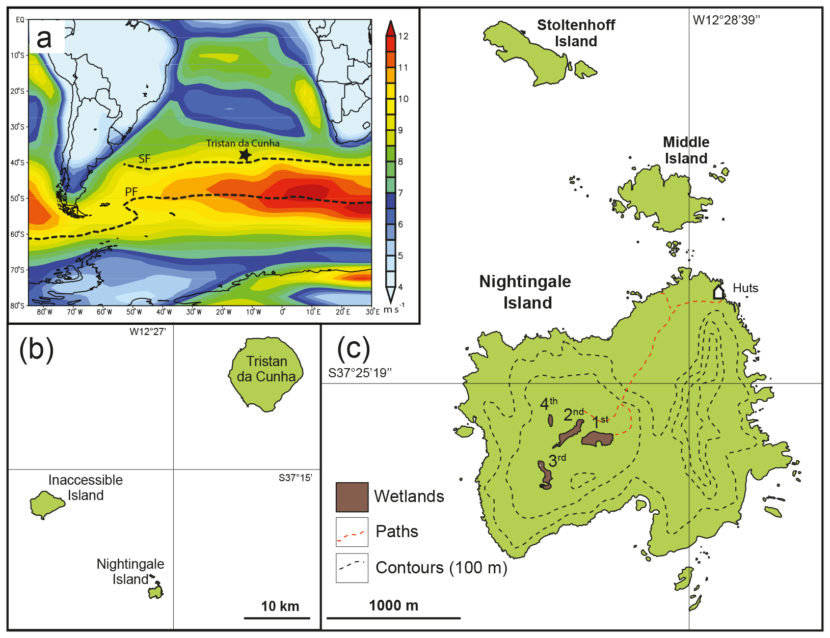
Figure 1(a) The position of the Tristan da Cunha island group in the South Atlantic and the 1000 mbar mean annual wind speed (m s−1) for 1980–2010 according to NCEP/NCAR reanalysis data showing yellow to red colors for the zone of the Southern Hemisphere westerlies, and the positions of the Subtropical Front (SF) and the Polar Front (PF) as dashed lines. (b) The three main islands of the Tristan da Cunha island group. (c) The position and size of the four overgrown lake basins, so-called ponds (labeled 1P–4P), on Nightingale Island with 100 m contour lines.
The Tristan da Cunha island group (TdC) at 37.1∘ S (Fig. 1) sits strategically at the northern boundary of the SHW (Fig. 1a), a few degrees north of the Subtropical Front (SF), where sea surface temperatures (SSTs) and salinities decrease by 3–4 ∘C and 0.3 ‰, respectively. Annual mean air temperature and precipitation are 14.3 ∘C and approximately 1500 mm, respectively, with highest precipitation in austral winter when the SHW impact is largest. The record presented here is from the 1st Pond (labeled 1P), an overgrown crater lake (200 m×70 m, 207 m a.s.l.) today forming a peat bog in the central part of Nightingale Island (NI) (Figs. 1 and 2), a volcanic island dominated by trachytic bedrock. Its drainage area is about twice the size of the peat bog and is thus sensitive to changes in the precipitation and evaporation balance (P/E). Previous studies from NI show that the area experienced shifts in precipitation during the Holocene (Ljung and Björck, 2007) and partly also during the Last Glacial Termination (Ljung et al., 2015), mainly attributed to the changing impact of the SHW. These data also indicate a southerly displacement of the Intertropical Convergence Zone (ITCZ) during the Heinrich 1 event (H1) and warming in the South Atlantic as a consequence of reduced AMOC, causing the lake basin to dry out, and create a hiatus between 18.6 and 16.2 ka (Ljung et al., 2015). Here we present a multiproxy study of the sediments that accumulated before this hiatus dating to 36.4–18.6 ka, covering the younger part of Marine Isotope Stage 3 (MIS 3) and most of MIS 2, a climatically very dynamic period with Antarctic Isotope Maxima (AIM), DO events and H events. In spite of its fairly northern position in relation to Antarctica, we hypothesize that TdC was impacted by such events in terms of shifts of SHW, which we aim to test by using a suite of proxies.
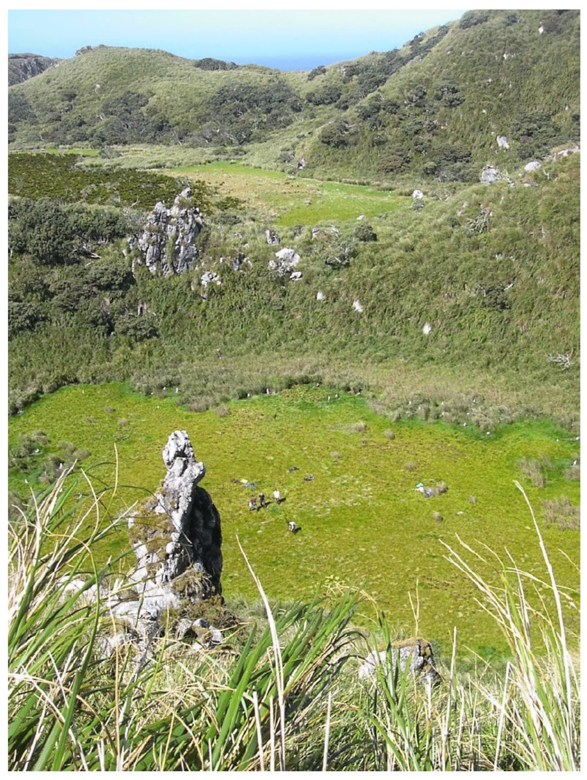
Figure 2Photograph from Nightingale Island. The overgrown lake basins of 1st Pond and 2nd Pond are shown, with the higher-situated 1st Pond in the background, seen towards the southeast. Note the albatross chicks (white dots) and the four people on 2nd Pond for scale. Photo Svante Björck.
A large set of proxy data were analyzed, including chemical (N, XRF (X-ray fluorescence) elemental concentrations and isotopes (13C, 15N, 2H or D)), biological (TOC (total organic carbon), molecular fossils such as n-alkanes, glycerol dialkyl glycerol tetraether lipids (GDGTs), pollen and diatom assemblages, and biogenic silica (BSi)), and physical (magnetic susceptibility (MS)) parameters. Some proxies provide information about local changes such as soil conditions and erosion (C∕N ratios, 13C and MS), weathering (major element data), vegetation composition (pollen, n-alkane distributions), organic productivity (TOC and BSi), lake conditions and levels (diatoms, BSi, δD values of short-chained n-alkanes), and bird impact (15N). Others display regional changes in hydroclimate, such as mean annual air temperature (MAAT) and mean summer air temperature (MST) from the GDGT lipids and the source water of terrestrial and aquatic plants including evaporative conditions (hydrogen isotopes, δD). Observations of the isotopic content of precipitation are very sparse around TdC, and therefore we have investigated the hydroclimate variability with an isotope-enabled climate model. In addition, we have performed principal component analysis (PCA) to distinguish the influence of the different proxies on samples (see Methods, Sect. 3.13). Most of our data are found in the Supplement.
3.1 Field work, handling of cores and sample collection
Two weeks of field work on NI were carried out in February 2010 and drilling was carried out using Russian chamber samplers providing 1 m long cores (∅=50 and 75 mm) with overlaps of 15–50 cm between each cored section. The ketch Ocean Tramp provided the transport from the Falkland Islands to TdC and back to Uruguay. In order to penetrate as deep as possible into the very stiff sediments, a chain hoist was used for coring the deeper parts of the sequences. The sediments were described immediately in the field before being wrapped in plastic film and PVC tubes. Upon arrival in Uruguay, the cores were transported to the Geology Department in Lund where they were stored in a cold room. Before subsampling for the different proxy analyses, the field-based lithostratigraphy and correlations between individual core sections were adjusted in the laboratory. This was aided by magnetic susceptibility (κ) measurements, which give a relative estimate of the magnetic mineral concentration, to confirm and adjust the visual correlation between overlapping core segments.
3.2 Radiocarbon dating and age model
The radiocarbon-dated material consisted of 1 cm thick, organic-rich, bulk sediment. All 41 dated samples were pre-treated and measured at the Lund University Radiocarbon Dating Laboratory with single-stage accelerator mass spectrometry (SSAMS). The age model (Fig. 3) was constructed using the OxCal software package (Bronk Ramsey, 1995, 2009a). To minimize subjective user input, we ran the age model with a general outlier model (Bronk Ramsey, 2009b) and a variable k value that lets the model itself determine the sedimentation rate variability (Bronk Ramsey, 2008). For calibration we use the Southern Hemisphere calibration data set, SHCal13 (Hogg et al., 2013).
3.3 Measurements for magnetic susceptibility
Magnetic susceptibility (κ) was measured using a Bartington MS2E1 high-resolution surface scanning sensor coupled to a Tamiscan automatic logging conveyor. Measurements were carried out on non-sampled half cores and with a resolution of 5 mm and with results shown in 10−6 SI units. The magnetic susceptibility gives a relative estimate of the ability of the material to be magnetized, i.e., the magnetic mineral concentration.
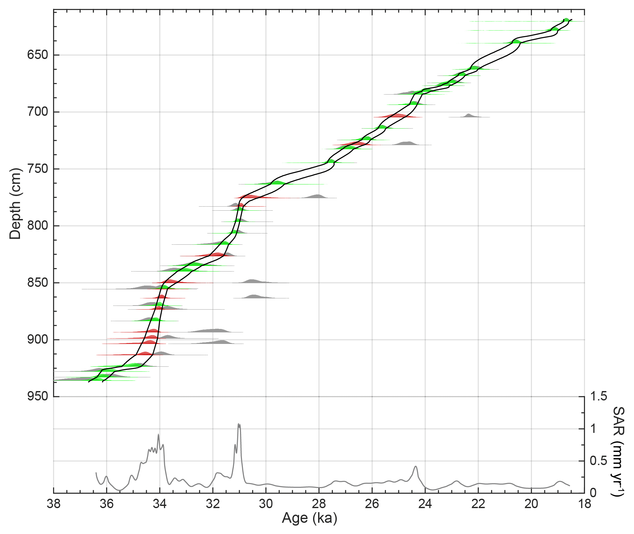
Figure 3Age model for the sediments at 1st Pond, Nightingale Island. Top plot: radiocarbon-based age–depth model (black lines encompass the 68.2 % probability interval). The patches indicate the calibrated probability distributions of each radiocarbon date for un-modeled (single) dates (gray patch) and their posterior distributions when modeled as a P sequence: green patches indicate agreement indices of > 60 % and red patches agreement indices of < 60 %, i.e., outliers. Bottom plot: sediment accumulation rates (SAR, mm a−1) based on the mean age–depth model shown in the top panel.
3.4 XRF analyses
A handheld Thermo Scientific portable XRF analyzer (h-XRF) Niton XL3t 970 GOLDD+ set to the Cu/Zn mining calibration mode was used. The instrumentation provides highly accurate determinations for major elements (Helfert et al., 2011). All analyses were performed on freeze-dried sediments from the 1P cores using an 8 mm radius spot size in order to obtain representative values. The elemental detection depends partly on the duration of the analysis at each point; this is especially true for the lighter elements such as Mg, Al, Si, P, S, Cl, K and Ca. For this reason the measurement time of each sample was set to 6 min. Although a larger suite of elements was acquired, we have chosen to work with Al, Si, P, S, K, Ca, Ti, Mn, Fe, Rb, Sr and Zr. These elements were selected based on their analytical quality (i.e., level above the detection limit) and with the help of principal component analysis (PCA). PCA was made using JMP 10.0.0 software in correlation mode using a Varimax rotation. Before analysis all data were converted to Z scores calculated as , where Xi is the normalized elemental peak areas and Xavg and Xstd are the series average and standard deviation, respectively, of the variable Xi. A Varimax rotation allocates the component variables which are highly correlated (sharing a large proportion of their variance) – imposing some constrains in defining the eigenvectors. By grouping together elements showing similar variation, the chemical signals tend to be clearer and key elements are better identified. To simplify the interpretation of our principal components (PCs) we employ a modified Chemical Index of Alteration (CIA), see Fig. 4d, as defined by Nesbitt and Young (1982): CIA . This index expresses the relative proportion of Al2O3 to the more labile oxides and is an expression of the degradation of feldspars to clay minerals. Since we have no NaO data, we call it a modified CIA.
3.5 C and N analyses
Dried and homogenized samples every 1–2 cm were analyzed with a Costech Instruments ECS 4010 elemental analyzer. The accuracy of the measurements is better than ±5 % of the reported values based on replicated standard samples. To account for C∕N atomic ratios, the ratio was multiplied by 1.167.
3.6 13C and 15N analyses
Dried, homogenized bulk samples were measured using a Thermo Fisher DeltaV ion ratio mass spectrometer. The isotopic composition of samples is reported as conventional δ values in parts per thousand relative to the Vienna Pee Dee Belemnite (13C) and atmospheric 14N (15N): δsample (‰) = [(Rsample−Rstandard)/(Rstandard)] ×1000, where R is the abundance ratio of 13C∕12C in the sample or in the standard.
3.7 Pollen analyses
Sixty-four levels were subsampled and analyzed for their pollen content. Pollen samples of 1 cm3 were processed following standard method A as described by Berglund and Ralska-Jasiewiczowa (1986) with added Lycopodium spores for determination of pollen concentration values. Counting was made under a light microscope at magnifications of 400× and 1000×. The aim was to count at least 500 pollen grains in every sample, which was almost achieved (mean sum of 565 pollen grains and mean sum of 870 pollen grains and spores). Identification of pollen grains and spores was facilitated by published photos (Hafsten, 1960), standard pollen keys (Moore et al., 1991) and a small collection of type slides from Tristan da Cunha borrowed from the University Museum of Bergen, the Natural History Collections. The pollen percentage diagram (Fig. 5) was plotted in C2 software (Juggins, 2007). Warm/cold pollen ratios were calculated as (), where warm pollen types (Wp) are from plants only found below 500 m a.s.l. and cold pollen types (Cp) are from plants only found above 500 m a.s.l.
3.8 Diatom analyses and diatom environmental ratios
One hundred and seventy-nine levels of 0.5 cm thick sediment segments were subsampled to analyze their diatom content. For preparation of diatom slides, ∼200 mg of freeze-dried sediment was oxidized with 15 % H2O2 for 24 h, then treated with 30 % H2O2 for a minimum of 24 h, and finally heated at 90 ∘C for several hours. A known quantity of DVB (divinylbenzene) microspheres was added to 200 µL aliquots of the digested and cleaned slurries in order to estimate diatom concentrations (Battarbee and Keen, 1982). The diatoms were mounted in Naphrax® medium (refractive index =1.65). Three hundred valves or more per sample were counted in most samples and identified largely using published diatom floras (Krammer and Lange-Bertalot, 1986; Le Cohu and Maillard, 1983; Moser et al., 1995; Van de Vijver et al., 2002). Diatom results are expressed as relative percent (%) abundance of each taxon (Fig. S3 in the Supplement) and also as total concentrations of valves per gram of dry sediment.
Freshwater diatom species are excellent indicators of water quality, particularly of pH, conductivity and dissolved nutrients (Battarbee et al., 2001). Sedimentary diatom assemblages inter alia can be used to reconstruct past changes in water quality using the ecological indicator information for each species. Where suitable modern diatom–water quality calibration data sets exist, transfer functions can be generated to reconstruct these changes. However, in sediment records where diatom diversity is low and affinities of some species are not firmly established, placing diatom taxa into ecological or environmental preference groups using literature attributions and field experience can be used to generate ratio scores relevant to past conditions. The 1st Pond assemblages are suitable for such an approach, particularly for inferring changes in habitat and water acidity. The acid diatom index ratio is derived from the sum of acid water indicating taxa comprising Aulacoseira, Frustulia, Pinnularia and Eunotia compared to that of the fragilarioid tychoplanktonic taxa. Proportions of acidity-tolerant to acidity-intolerant diatom taxa indicate water pH; total tychoplankton (temporary phytoplankton) vs. total benthic taxa relate to open-water conditions; subaerial and terrestrial taxa vs. the total assemblage indicate wetland development and/or in-washed material.
3.9 Biogenic silica analyses
The 310 samples were analyzed using a wet-alkaline digestion technique (Conley and Schelske, 2001). Samples were freeze-dried and gently ground prior to analysis. Approximately 30 mg of sample was digested in 40 mL of a weak base (0.47 M Na2CO3) at 85 ∘C for a total duration of 3 h. Subsamples of 1 mL were removed after 3 h and neutralized with 9 mL of 0.021 M HCl. Dissolved Si concentrations were measured with a continuous-flow analyzer applying the automated molybdate blue method (Grasshoff et al., 1983). Biogenic silica content in lake sediments is a rough proxy for lake productivity.
3.10 Lipid biomarker and compound-specific hydrogen isotopic analyses
The hydrogen isotopic composition (δ notation) of n-alkanes was analyzed by gas chromatography isotope ratio monitoring mass spectrometry (GC-IRMS) using a Thermo Finnigan Delta V mass spectrometer interfaced with a Thermo Trace GC 2000 using a GC Isolink II and Conflo IV system. Helium was used as a carrier gas in constant flow mode and the compounds separated on a Zebron ZB-5HT Inferno GC column (30 m × 0.25 mm × 0.25 µm). Lipid extraction was performed on freeze-dried samples by sonication with a mixture of dichloromethane and methanol (DCM–MeOH 9:1 v∕v) for 20 min and subsequent centrifugation. The process was repeated three times and supernatants were combined. Aliphatic hydrocarbon fractions were isolated from the total lipid extract using silica gel columns (5 % deactivated) that were first eluted with pure hexane (F1) and subsequently with a mixture of DCM–MeOH (1:1 v∕v) to obtain a polar fraction (F2). A saturated hydrocarbon fraction was obtained by eluting the F1 fraction through 10 % AgNO3−SiO2 silica gel using pure hexane as eluent. The saturated hydrocarbon fractions were analyzed by gas chromatography mass spectrometry for identification and quantification, using a Shimadzu GCMS-QP2010 Ultra. C21 to C33 n-alkanes were identified based on mass spectra from the literature and retention times. The concentrations of individual compounds were determined using a calibration curve made using mixtures of C21–C40 alkanes of known concentration. More details about the GC-IRMS method, including GC oven temperature program, instrument performance and reference gases used, are given in Yamoah et al. (2016). The average standard deviation for δD values was 5 ‰. Due to low sea levels during the time period of our proxies, the δD values of the n-alkanes were ice volume corrected (Tierney and deMenocal, 2013), δD, with interpolated ocean water δO values (Waelbroeck et al., 2002).
Isoprenoid and branched glycerol dialkyl glycerol tetraethers (GDGTs) were measured on the F2 fractions after filtration through 0.45 µm PTFE filters and reconstitution into a known volume of methanol. Analysis was done using a Thermo–Dionex HPLC (high-performance liquid chromatography) connected to a Thermo Scientific TSQ Quantum Access triple quadrupole mass spectrometer, using an APCI (atmospheric pressure chemical ionization) interface. Chromatographic separation was achieved using a reverse phase method similar to the one used by Zhu et al. (2013). Partially coeluting GDGT isomers were integrated as one peak in order to obtain data comparable to the normal phase method that has been in use by the community since Weijers et al. (2007).
A basic prerequisite for the valid use of brGDGTs (branched GDGTs) is a relatively high branched-over-isoprenoid tetraether (BIT) index, which was 1.00 throughout the core. Reconstructed pH values, based on the cyclization of branched tetraether (CBT) ratio (Weijers et al., 2007), were stable at 6.6±0.1 over the length of the core, which means that temperature is the dominant environmental factor exerted on the brGDGT distribution. At the time of measurement, we had not adopted the new method which separates between 5-methyl and 6-methyl branched GDGTs (De Jonge et al., 2014). As a consequence, we do not have individual quantifications of 5-methyl and 6-methyl branched GDGT isomers needed to use the revised 5-methyl branched tetraether (MBT5me) temperature proxy for mineral soils (De Jonge et al., 2014) or peat (Naafs et al., 2017), which gives lower root-mean-square error than the original terrestrial (soil) calibration (Weijers et al., 2007). However, since our data are from lake sediments, we argue that GDGT-based temperature proxy calibrations based on lake surveys is in any case a more valid approach. Indeed, using the original temperature calibration of Weijers et al. (2007) based on soils resulted in very low temperatures between 0 and 6 ∘C, a cold bias observed in other studies from lakes. This bias is probably due to the addition of in situ produced brGDGTs on top of any brGDGTs eroded from land (Loomis et al., 2012; Pearson et al., 2011). Our record could be biased by a changing ratio of soil- and lake-derived GDGTs, where a greater relative contribution of terrestrial-derived GDGTs would result in a warm bias if a lake calibration is used. However, we do not find a correlation between GDGT-derived temperature and two proxies for terrestrial influx, the C∕N ratio and magnetic susceptibility, but rather the opposite. We used two lake calibration sets: (a) the one of Pearson et al. (2011), based on a global lacustrine data set and using mean summer temperatures (MST), including samples from nearby South Georgia island in the South Atlantic, and (b) a calibration based on a large data set of east African lakes from different altitudes (Loomis et al., 2012), using mean annual air temperatures (MAAT), and which is also applicable outside of east Africa (Loomis et al., 2012). It is impossible to test which of these two proxy records would reflect past conditions more accurately. However, the two reconstructions strongly covary, with a difference between reconstructed MST and MAAT of approximately 5 ∘C.
3.11 Calculation of insolation values
A long-term numerical solution for earth's insolation quantities (Laskar et al., 2004) was used for the insolation values, 37–18 kyr at 37∘ S, and calculated with the AnalySeries program. While the austral winter values were based on mean daily June–August insolation (W m−2), the mean austral summer values were based on the mean daily December–February insolation.
3.12 Isotope model simulation
The isotope model analysis is based on a 1200-year simulation using the isotope-enabled version of the ECHAM5/MPI-OM earth system model (Werner et al., 2016) run with natural and anthropogenic forcings for 800 to 2000 CE (Sjolte et al., 2018). Horizontal resolution of the atmosphere is (T31) with 19 vertical layers, while the ocean has a horizontal resolution of with 40 vertical layers. The model includes isotope fractionation for all phase changes in the hydrological cycle, including below-cloud evaporation. Since both the present-day situation and our Nightingale Island record show a continuous impact from the westerlies, we deem it valid to use this late Holocene simulation as an analog for interpreting the variability in the westerlies during the time period of study. The outcome of the simulation is presented in the results section but further investigation of the model run shows that the multidecadal variability in δD at TdC is related to the phase of the Southern Annular Mode, indicating that isotopic variability at TdC is sensitive to large-scale SH climate variability (Fig. S4).

Figure 4Antarctic ice core data and some proxy data from the sediments in 1st Pond between 36.4 and 18.6 ka. (a) The EPICA Dome Dronning Maud Land (EDML) δ18O record (EPICA Community Members, 2006) showing AIM7–2. (b) GDGT-based mean annual air temperature (MAAT) and mean summer temperature (MST) calibrated to Pearson et al. (2011) and Loomis et al. (2012), respectively. (c) Warm pollen ratios, percent (%) Phylica arborea pollen and percent (%) Ophioglossum spores. (d) Modified chemical index of alteration (CIA). (e) Percent (%) Cyperaceae pollen and n-C23 alkanes. (f) δD values (‰) of n-C23 and n-C27−31 alkanes. (g) Acid diatom ratios. (h) Percent (%) terrestrial diatoms. (i) Open water diatom ratios. (j) Percent (%) biogenic silica (BSi). (k) C∕N ratios. (l) % total organic carbon (TOC). (m) Magnetic susceptibility (MS) expressed as 10−6 SI units. All proxies relate to the age scale on the x axes. Note the two thick gray lines (31 and 26.5 ka) indicating the position of the three PCA zones (Fig. 6).
3.13 Principal component analysis (PCA)
PCA was performed with 14 of our proxies (Fig. 6b) that we expect to respond to hydroclimate changes but without the MAAT values in order to test the MAAT values vs. other climate proxies, using the C2 program (Juggins, 2007). The aim was to display the impact of different combinations of proxies on the samples in a biplot (Fig. 6b), as discussed below in Sect. 4.2. All proxy data were centered and standardized before calculation.
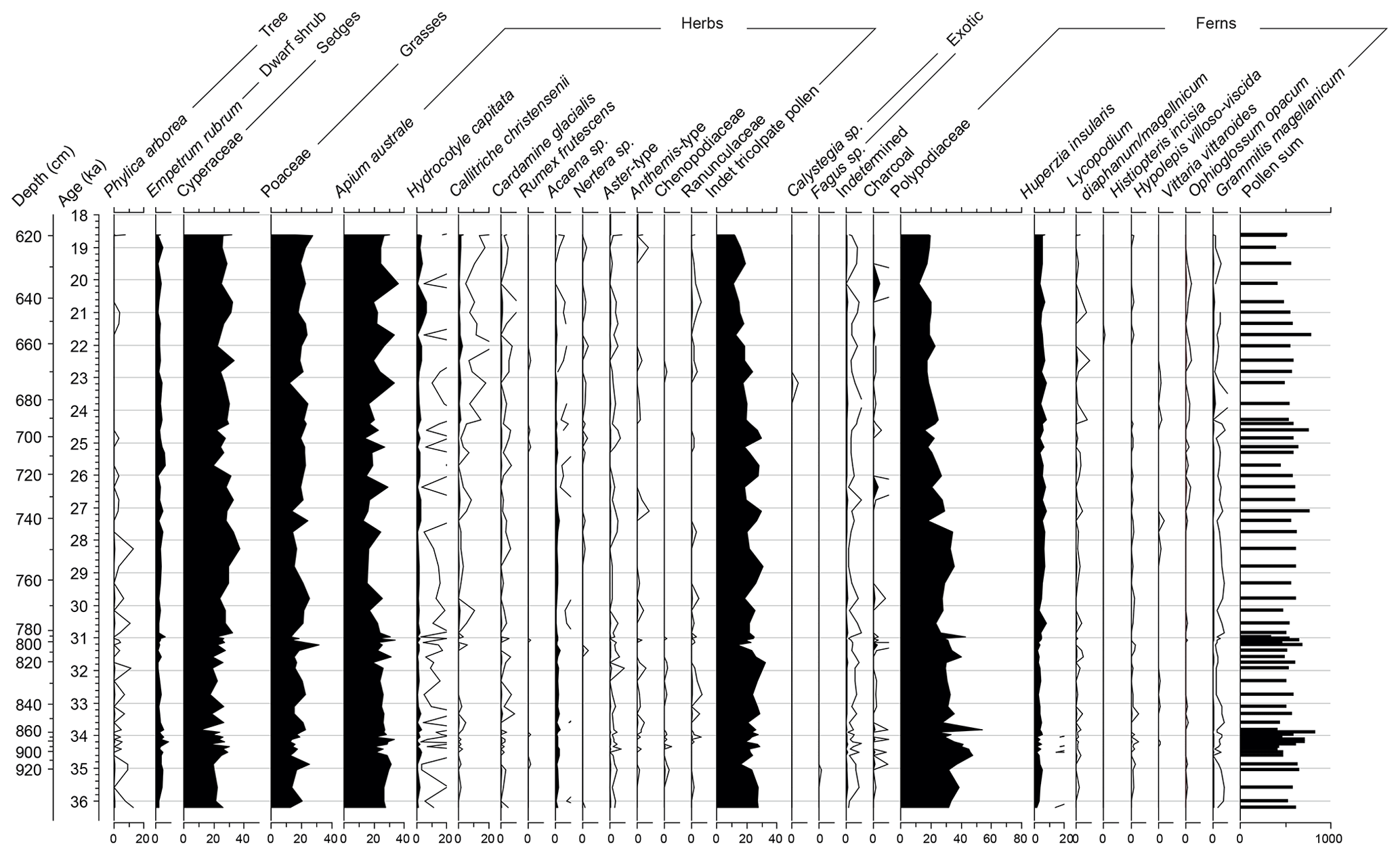
Figure 5Pollen diagram from 1st Pond, Nightingale Island. The diagram shows relative abundance (%) of the pollen taxa. Note that it is both related to depth (cm) and age (ka) on the y axis, the latter according to the age–depth model in Fig. 3.

Figure 6Principal component analysis (PCA) of 14 proxies from 1st Pond. (a) Scores of the first two principal components related to age and the three PCA zones. Note that negative values point upwards and how PC1 and PC2 values are related to temperatures and SHW to the right y axis. (b) PCA plot shows the loadings of the 14 proxies (shown as red dots and black text with reference to proxies in Fig. 4, except for Empetrum rubrum). PC1 (red-brown) and PC2 (blue) account for 38.1 % and 13.4 % of the variance, respectively. The interpretations of the two axes are shown by red-brown and blue texts, and the interpretations of the four segments are based on the combined positions of the proxies in the plot (shown in four different colors).
4.1 An island record of glacial climate in the central South Atlantic
Thirty-nine 1 m long overlapping cores were taken in February 2010 from three overgrown crater lakes (Fig. 1c) between lava ridges (Anker Björk et al., 2011). The 1st Pond (1P) was exceptional in that it was the only site where sediments older than 18.6 kyr were recovered. At 1P the 16.2–18.6 kyr hiatus (Ljung et al., 2015) is marked by a thin silt lamina at 618.8 cm. We retrieved five overlapping cores below the hiatus with 318.2 cm of sediments before coring was obstructed at 937 cm by suspected bedrock or boulders. These cores were correlated by lithology and magnetic susceptibility (MS). The lower 162 cm consists of a dark-brown slightly silty gyttja, overlain by a gray-brown silty clay gyttja, all deposited under anaerobic conditions. Because of the low concentration of plant macro-fossil remains our chronology is based on 41 14C dates of 1 cm thick bulk sediment samples between 620 and 936 cm (Table S1 in the Supplement). Comparisons of 14C dates of bulk sediment and plant remains (wood and peat) have shown good concordance (Ljung et al., 2015; Ljung and Björck, 2007), and the most likely explanation for the seven clear outliers (Fig. 3) is possibly a combination of statistical noise and contamination from small amounts of recent material. Our age model displays a mean sedimentation rate of 0.18 mm yr−1 but with considerable variation.

Figure 7Zonal mean changes in wind, temperature and precipitation related to δD variability at TdC. (a) Time series of simulated precipitation-weighted annual mean δD at TdC, with values above and below the 95th percentile indicated with red and blue circles, respectively. This selection of high and low δD is used to define the data in (e–g). (b–d) Annual modeled (black) South Atlantic zonal mean (30 to 0∘ W) westerly wind speed (850 mbar U wind, positive towards east), 2 m temperature (T2m) and precipitation compared to the 20th Century Reanalysis climatology 1981–2010 (gray) (Compo et al., 2011). (e–g) Composites of annual modeled zonal mean (30 to 0∘ W) westerly wind speed (850 mbar U wind), 2 m temperature (T2m) and precipitation for high (red) and low (blue) δD at TdC defined in (a). (h–j) High minus low anomalies of model output are shown in (e)–(f). Circles indicate significant anomalies (p < 0.01) calculated using two-tailed Student's t test. The vertical bars in (b)–(j) show the latitude of NI at 37∘ S.
In agreement with the supposed minimum age of pond formation through volcanic activity (Anker Björk et al., 2011), the bottom of 1P has an age of 36.4±0.3 ka. Our temperature records (Fig. 4b) show an oscillating pattern, with the largest change at 27.5 ka, and share similarities with the low-frequency variability in the EPICA Dome Dronning Maud Land (EDML) curve (Fig. 4a). Before 27.5 ka, MAAT and MST vary between 17 and 12 ∘C and between 21 and 17 ∘C, respectively, while the variation is between 13 and 9 ∘C and between 18.5 and 15.5 ∘C, respectively, after 27.5 ka. In terms of pollen as a local temperature indicator, it is known that Phylica arborea, Acaena sarmentosa and two Asteraceae plant types are sensitive to cold conditions (Ryan, 2007). They make up warm pollen types at NI, and the warm/cold pollen-types ratio (Fig. 4c) shows large variations until 31.4 ka, followed by a two-step decline (at 31.2 and 26.5 ka) largely in contrast to the spore abundance of the cold tolerant Ophioglossum opacum fern, and with a trend similar to the temperature curves. In comparison to Holocene sediments from NI (Ljung and Björck, 2007), the glacial pollen record from 1P (Fig. 5) shows less variability, and the most distinct difference is the very low abundance of the only tree species pollen on the island, the frost-limited P. arborea. Based on lapse rates, with 65–130 m lower sea levels during 35–18 ka (Lambeck et al., 2014), and today's distribution of P. arborea on TdC and Gough Island (Ryan, 2007), we can estimate that its absence after 28 ka implies minimum winter temperatures at least 3 ∘C lower than today, which agrees well with our MAAT curve (Fig. 3b).
To evaluate changes in the degree of weathered material, we used a modified Chemical Index of Alteration (CIA) (Fig. 4d). The long-term development can be divided into three phases with initially low but very variable values until 31 ka, a second phase with stable intermediate CIA values until 27 ka, followed by higher and varying values (Fig. 4d). Magnetic susceptibility (MS) shows centennial–millennial oscillations superimposed on an increasing trend from the bottom to the top of the core (Fig. 4m), which is an indicator of in-washed mineral matter from magnetite-rich basaltic rocks of the catchment. The values of total organic carbon (TOC) and biogenic silica (BSi) (Fig. 4l and j) reflect organic and aquatic productivity in and around the lake with highest values in the oldest section. TOC shows a general decline and BSi oscillates with higher values until 28 ka, after which it gradually drops. The fairly high C∕N ratios (Fig. 4k), with a mean value of 17.6, show that organic matter is a mix of terrestrial and aquatic sources. The high and oscillating ratios in the older section followed by a gradual decline implies terrestrial sources dominating until 28 ka, after which time aquatic sources become more important. With respect to bulk stable isotopes (Fig. S1), the high δ15N values imply a marine influence possibly related to the presence of marine birds (Caut et al., 2012), such as great shearwater and albatrosses, which have a great impact on the ponds today. Rising δ13C values at 25.7 ka are consistent with the declining C∕N ratios after 28 ka, i.e., more aquatic material with enriched 13C and perhaps in combination with a higher influence from C4 grasses.
Unlike the pollen record (Fig. 5), the diatom record shows large shifts and the 33 diatom taxa (Fig. S2) have been classified into three environmental forms. Changes in these groups imply shifts in aquatic and environmental conditions in and around the lake. They show a lake with open water early in the record, followed by shifting lake levels between 35 and 33 ka (Fig. 4i), supported by δD values of long- and mid-chain n-alkanes (Fig. 4f). At 31 ka the open-water ratios drop and reach a minimum at 29 ka, in antiphase with the acid water diatom ratios (Fig. 4g), followed by a rise until 26.6 ka. Thereafter acid species dominate as oligotrophic wetland encroached around the lake, while periods of more terrestrial diatoms imply episodes of in-washed diatoms from the surroundings. Around 21.2 ka more open-water conditions prevail again with high ratios during 19–18.6 ka, before the lake dried out (Ljung et al., 2015). The shifts in diatom communities show that 1P went through substantial hydrologic changes, some of which were rapid, induced by changing P∕E ratios, in contrast to the fairly stable vegetation around the lake as seen in the pollen record.
4.2 Linking the Nightingale Island record to South Atlantic hydroclimate
The hydrological sensitivity of a basin like 1P makes it ideal to place local changes into the context of regional hydroclimate shifts. To analyze the variability through time Principal component analysis (PCA) was carried out on a data set with 14 hydroclimate-sensitive proxies resulting in three PCA zones (Fig. 6a). Note that the resolution of the PCA record depends on the proxy with least common sample levels (Table S2), in this case biomarker analyses. Therefore the temporal resolution of the PCA is not as high as some ice core and marine records. Based on the proxy loadings in the PCA plot (Fig. 6b), it can be divided into four different segments with variable hydroclimate and environmental conditions. The importance of presumed temperature proxies on Axis 1 (38.1 % of the variance) is evident where warm pollen ratios, Phylica arborea pollen, BSi, TOC and open-water diatoms show warm humid conditions to the left (negative) in the biplot (Fig. 6b) vs. cooler and drier to the right. The latter is accentuated by Ophioglossum spores, a fern growing at high and cold altitudes on TdC. A correlation analysis between the PC1 values and our MAAT values (Fig. 4b) shows an r2 value of 0.56, corroborating that Axis 1 mainly represents temperature. Axis 2 (13.4 % of the variance) is linked to hydrologic indicators being dominated by the δD values of the aquatic n-C21−23 and terrestrial n-C27−31 alkanes (Fig. 6b). We interpret higher δD values (positive Axis 2 values) to show stronger influence of more local air masses, with more evaporation and semiarid conditions, also shown by Empetrum rubrum pollen in the upper left quadrant, while the upper right quadrant of the plot shows an acid oligotrophic swampy setting. The segment to the lower right in Fig. 6b displays cold conditions and in-wash of terrestrial diatoms as an effect of higher lake level during episodes of more precipitation. The lower left represents warm and wet conditions, implied by P. arborea pollen and open-water diatoms and, in general, negative Axis 2 values relate to more negative δD values.
To illustrate the relation between the position of the westerlies and the isotopic composition of precipitation at TdC in the simulation, we selected extreme values of high and low δD at TdC (Fig. 7a) and made composite anomalies of the annual mean westerly wind strength at 850 mbar (u850mb, Fig. 8a), precipitation (Fig. 8b), 2 m temperature (t2m, Fig. 8c) and precipitation-weighted δD (Fig. 8d) for high minus low δD at TdC. This shows that the variability in δD in precipitation at TdC is only weakly dependent on local temperature. Instead, shifts in δD at TdC are related to large-scale changes in precipitation and the position of the westerlies. Positive δD anomalies at TdC imply a more southern position of the core of the westerlies with drier and more subtropical conditions at TdC, and negative δD anomalies at TdC denote a more northern position of the core of the westerlies bringing more polar air masses with wetter conditions at TdC. From Figs. 7 and 8, we note that the shifts in TdC precipitation are governed by the precipitation zone on the northern flank of the westerlies shifting with the position of the westerlies themselves. We therefore conclude that our model analysis shows that isotope variability in precipitation at TdC is mainly related to shifts in large-scale circulation. High δD values at TdC imply a more southerly SHW position with stronger winds in its core, while low δD values show a more northerly SHW position with weaker winds (Fig. 7e and h). Our analysis also shows that high (low) δD values are related to less (more) precipitation at TdC but shows little dependency on temperature (Figs. 7f and i, and 8c). The amplitudes of the δD values in our proxies are significantly larger than the modeled amplitudes, implying larger changes in the climate variables during the recorded isotope shifts compared to the year-to-year variability in the model. Furthermore, the modeled relationship between δD and precipitation corresponds well to the PC2 variability in the proxies (Fig. 6b); for example, high PC2 and δD values relate to more Cyperaceae (lake overgrowth) and Empetrum pollen values (arid soils) and more acid diatoms (swampy), while low PC2 values relate to open-water (lake) and terrestrial (flushed-in) diatoms.
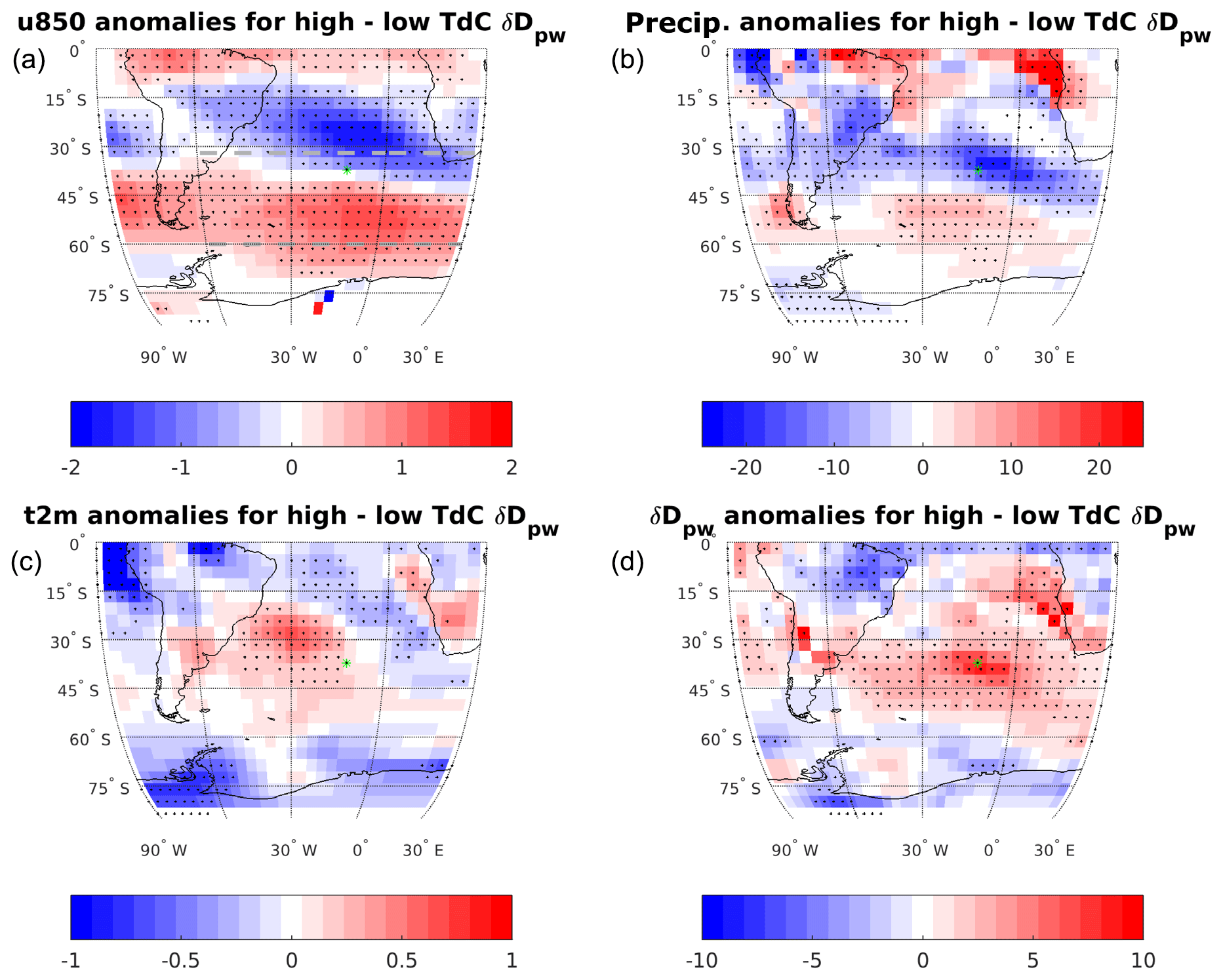
Figure 8Composite maps of changes in wind, precipitation, temperature and δD related to δD variability at TdC, showing annual anomalies based on composites for high and low δD at TdC (see Fig. 7a). (a) Westerly wind speed (850 mbar U wind, positive towards east (m s−1)). The dashed gray lines show the approximate northern and southern boundaries of the westerlies (850 mbar U wind > 5 m s−1) to clarify that high TdC δD is related to a southwards shift in the westerlies. (b) Precipitation (mm month−1). (c) 2 m temperature (t2m (∘C)). (d) Precipitation-weighted δD (‰). Stippling indicates significant anomalies (p < 0.01) calculated using a two-tailed Student's t test. The green spot shows the position of TdC.
5.1 The large-scale hydroclimate pattern
The three PCA zones, dated to 36.2–31.0, 31.0–26.5 and 26.5–18.6 ka, show a trend and pattern which is recognizable in much of our data set as well as in the EDML (Fig. 4a) and South Atlantic marine record (Fig. 10b). Zone 1 is fairly warm but oscillates between low and high PC2 values, related to more northerly and weaker SHW, and more local air masses with stronger westerlies in a more southern position, respectively. Zone 2 is generally more stable with some minor oscillations with more southerly SHW and corresponds largely to the fairly warm period in Antarctica with the three isotope maxima, AIM4.1, AIM4 and AIM3 (Fig. 4a), and a stable and mild period in the South Atlantic marine realm (Fig. 10b). Zone 3 shows a cooling trend, also visible in the EDML and marine record, with variable SHW. It appears that TdC was continuously influenced by the SHW, as shown by the absence of arid conditions and generally low δD values, verified by humid conditions in southwestern-most Africa throughout most of MIS3 and MIS2 (Chase and Meadows, 2007). Apart from the resemblance between the long-term trends in Antarctic ice core data and marine data at 41∘ S in the South Atlantic (Barker and Diz, 2014) with our data it is, in spite of our lower resolution, interesting to compare our PC2 and δDn-CC27−C31 records (Figs. 4a and 10g) with other regional records related to SHW. Taking age uncertainties in a few hundred years into account we note a resemblance with marine Fe fluxes at 42∘ S (Martínez-García et al., 2014) where low δD values (Fig. 10g) covary with high Fe fluxes (Fig. 10f) due to northerly SHW in a cooler Southern Hemisphere, thus expanding the Patagonian dust source. Similar covariability can be seen in the δ18O record on fluid inclusions of SE Brazilian speleothems (Millo et al., 2017), where low values (Fig. 10e) imply strengthening of the monsoon shifting the South Atlantic atmospheric system southwards, including SHW. We also note that the Antarctic CO2 record (Fig. 10c) and the record (Gottschalk et al., 2015) from the South Atlantic (Fig. 10d), inferring AMOC strength and Southern Ocean ventilation, share similarities with our SHW records, described in the section below.

Figure 9Parametric plot of the PC1 and PC2 sample values as a function of time shown by the color bar to the right. Red numbers denote each age with gray numbers at the start and end of the plot. Data were interpolated to 50-year time steps to illustrate rate of change; the larger the distance between dots, the more rapid the change. Note that the hydroclimate interpretations from Fig. 6b are shown on the two PC axes.
5.2 A detailed hydroclimate scenario for the central South Atlantic
Due to chronological uncertainties in all records, lower resolution in some records and the complex phase relationships during abrupt interhemispheric climate shifts (Markle et al., 2016), detailed comparison of short-term variations across sites has to be treated with caution. In spite of these short-comings we will present a scenario based on our record and likely correlations.
The start of our record shows warm and wet conditions with northerly SHW, coinciding with the long and warm AIM7 followed by a cooling (Fig. 10j) at the onset of DO7. This is followed by the very dynamic period, 35–33 ka, shown by high sedimentation rates (Fig. 3) and peak variability in terms of both rapidity and amplitude (Fig. 9). Such variability is also seen in marine and ice core records, and in spite of the age uncertainties at 34–35 ka (Fig. 3) we tentatively correlate this period in our record to the end of DO7 and the minimum between AIM6 and AIM7. This corroborates the overlaps and time lags that have been postulated for DO and AIM events (Markle et al., 2016; Pedro et al., 2018; WAIS Divide Project Members, 2015). At 34 ka we note a temperature peak at the onset of AIM6 (Figs. 4 and 11) followed by falling temperatures, δD, Fe flux and CO2 values and high humidity (Fig. 10g, f, c and h). This change reflects northerly and weaker westerlies, with rising speleothem δ18O and West Antarctic Ice Sheet (WAIS) dln values (Figs. 10e and 11e), denoting the start of DO6 with a warming of the NH (Fig. 10a). This caused a northwards-shifting ITCZ and SHW in line with the theory that the atmospheric circulation system moves towards the warmer hemisphere, responding to the change in the cross-equatorial temperature gradient (McGee et al., 2014). At 33.5 ka we see a southwards SHW shift with rising temperatures and higher CO2 and lower WAIS dln values with dry conditions. We relate this to the onset of AIM5: a warming which is interrupted at 32.8 ka by a northerly SHW shift and wetter conditions (Figs. 11f and 10h) possibly triggered by DO5. This partly continues until 31.7 ka when SHW move south with a minor temperature rise (Fig. 11d) and decreasing humidity, possibly as a response to the post-DO5 cooling (Fig. 10a). The high variability and large amplitude of the changes in Zone 1 (Fig. 9) have facilitated conceivable correlations to other records. Based on these results we can conclude that the variability of PC2 implies a northerly shift of the SHW and a more southerly position during warm periods in Antarctica, also in line with interpretation of Antarctic deuterium excess data (Markle et al., 2016).
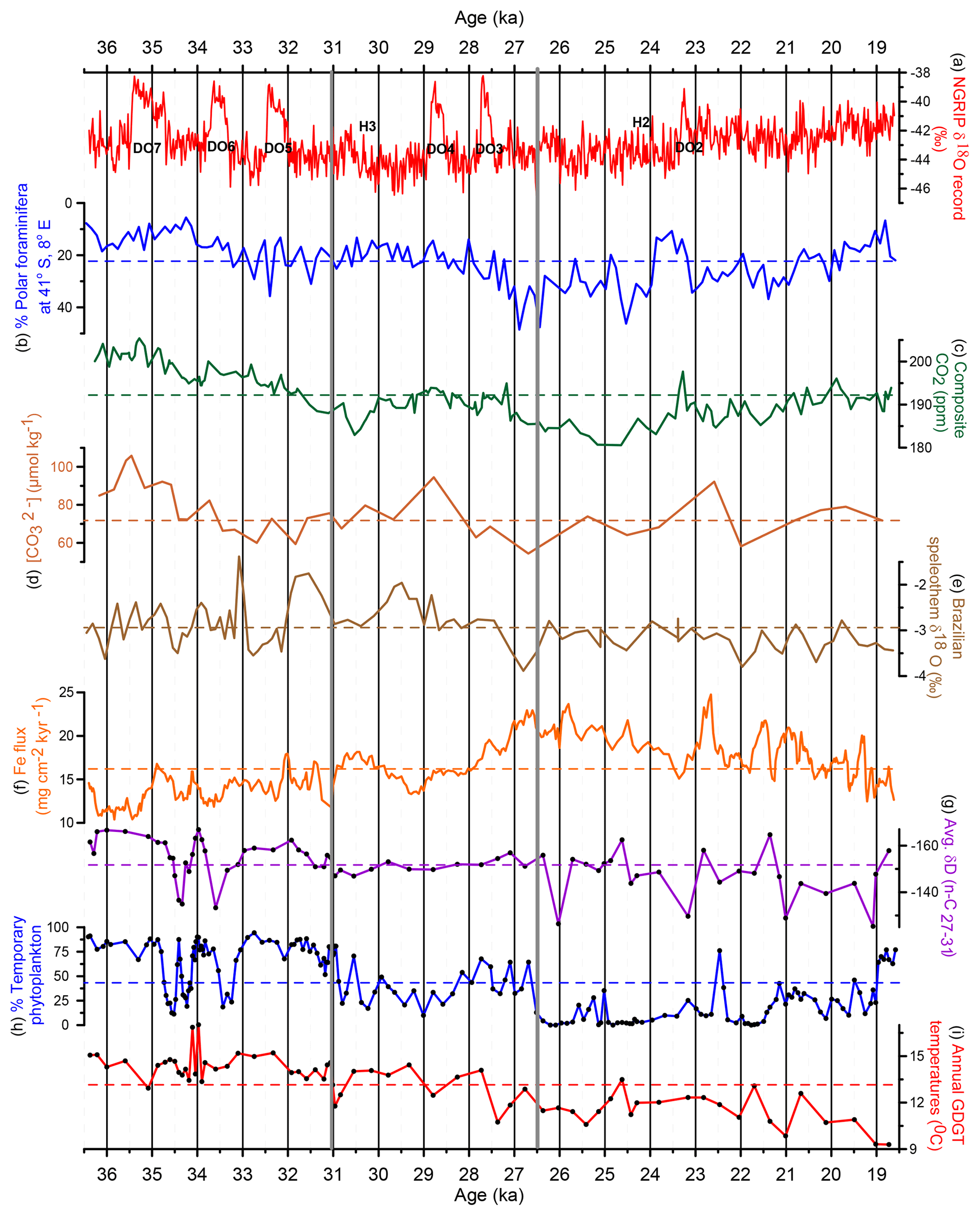
Figure 10Comparisons between other proxy records (a–f) and Nightingale Island proxies for SHW (g), wetness (h) and temperature (i), with mean values as broken lines. (a) δ18O values from the North Greenland Ice core Project (NGRIP) ice core (Andersen et al., 2006) showing DO and H events. Ice core records are on a common timescale (Veres et al., 2013). (b) Abundance (%) of polar foraminifera at 41∘ S in the South Atlantic (Barker and Diz, 2014). (c) Composite Antarctic CO2 record from Siple Dome (Ahn and Brook, 2014) and WAIS (Stenni et al., 2010). (d) () data at 44∘ S in the South Atlantic (Gottschalk et al., 2015). (e) Speleothem 18O record on fluid inclusions from SE Brazil (Millo et al., 2017). (f) Fe flux data in the South Atlantic at 42∘ S (Martínez-García et al., 2014). NI data are then followed. (g) Average δD values for the terrestrial n-C27−31 alkanes. (h) Abundance (%) of temporary phytoplanktonic diatoms implying relative water depth. (i) MAAT from the GDGT analyses. Note that sample levels are shown by a dot in (g)–(i) and that y axes of (b) and (g) show higher values downwards to facilitate comparisons to other proxies. Note that the two thick gray lines (31 and 26.5 ka) indicate the position of the three PCA zones (Fig. 6).
The Zone 1–Zone 2 boundary at 31 ka (Fig. 6a) is a dynamic transition, shown by many proxies and peak sedimentation rates (Figs. 9 and 3). The 4.5 kyr long and stable Zone 2 (Fig. 6a) is characterized by fairly high but slightly decreasing temperatures and, as in Zone 1, a dominating southerly SHW position. It is possible, taking age uncertainties into account, that H3 at 30.5 ka (Fig. 10a) triggered the southbound SHW, the rising CO2 and MAAT values, and the reduced humidity between 31 and 30 ka (Figs. 11f, 10c, 10i and 10h). The following long and warm AIM4 may have stabilized conditions in the South Atlantic in spite of the DO4 event at 28.8 ka. This stability is also seen in marine records (Fig. 10b), and the rather stable southern position of the SHW agrees with the fairly high CO2 values between 30 and 27.2 ka and with falling and rather low Fe fluxes (Fig. 10f). We also note higher lake evaporation from δD values of the aquatic n-C23 (Fig. 4f) in concert with rising summer insolation (Fig. 11a). Around 27.5 ka we see a brief response in some of the proxies to the short DO3 event (Fig. 10a), such as the MAAT and PC2 records (Fig. 11d and f), which is also noticeable in, for example, the marine and Brazilian monsoon records (Fig. 10b and e).
The start of Zone 3 at 26.5 ka (727 cm) constitutes the most drastic change in our record (Figs. 6a and 9) but timing varies between proxies (Fig. 4). MAAT, TOC and C∕N ratios start to decrease already at 28–27.5 ka, coinciding with DO3, while the biologic proxies (Figs. 4C and g–j, S2) respond slightly later possibly because they do not react until certain hydroclimate thresholds for the vegetation and algae flora are reached. The Zone 2–Zone 3 transition is roughly simultaneous with the onset of LGM in Antarctica (Fig. 10c), when 1P switched from a lake to a wetland, coinciding with increased abundance of polar foraminifera at 41∘ S (Fig. 10b). This may be an effect of the SF moving north of TdC, a meridional shift comparable to what has been shown from the eastern Pacific (Kaiser et al., 2005). The fairly stable PC1 values show cool and less-humid LGM conditions, while the variable PC2 values imply shifts in the position of SHW (Fig. 11f). There is also some correspondence between our δD (n-C27−31) maxima after 27 ka and Fe flux minima from the South Atlantic (Fig. 10g–f), both indicating southerly shifts of SHW. During this period our data also show generally higher mean δD (n-C27−31) values than in Zone 1, implying a more southern position of SHW during the Antarctic LGM, as seen in some modeling results (e.g., Sime et al., 2016). This is also compatible with the fact that the LGM temperature lowering in the Northern Hemisphere (Johnsen et al., 1995) was much larger than in the south (Stenni et al., 2010), shifting the atmospheric system to the south due to changes in the cross-equatorial gradient (McGee et al., 2014), also implied by the speleothem δ18O data (Fig. 10e) showing increased precipitation (Millo et al., 2017).
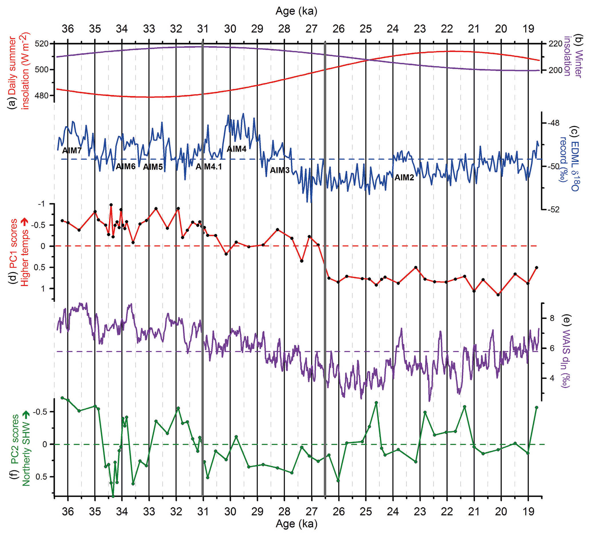
Figure 11Comparison between our PC1 and PC2 records and other relevant data. (a, b) Mean daily summer and winter insolation at 37∘ S (Laskar et al., 2004). (c) EDML δ18O record (EPICA Community Members et al., 2006) with Antarctic Isotope Maxima (AIM). (d) PC1 scores implying temperature shifts at NI. (e) WAIS dln values from west Antarctica (Markle et al., 2016). (f) PC2 scores indicate impact of SHW at NI. Note that sample levels, i.e., time resolution, for the PC records are shown as dots. Note the two thick gray lines (31 and 26.5 ka) indicating the position of the three PCA zones (Fig. 6).
After 26.5 ka we note phases of less-humid swampy oligotrophic conditions on NI at 26, 24.5–23, 22 and 20.5–19 ka (Fig. 10h) interrupted by periods of more or less open water, possibly driven by shifts of SHW. The former often show enriched δD values (Fig. 10g), while the latter were characterized by higher precipitation and more depleted δD values. Regarding the response of CO2 to these SHW shifts, we note a fairly good agreement between low/falling CO2 values and a northerly SHW position, and vice versa. For example, the CO2 minimum at 24.5–25 ka (Fig. 10c) matches with an extreme northern SHW position (Figs. 10g and 11f), and the CO2 peak at 23.3 ka agrees with the end of a long phase of southwards-moving SHW. The latter might have been triggered by the onset of H2 at 24.1 ka (Fig. 10a) followed by the inception of AIM2 (Fig. 11c).
The absence of P. arborea (Figs. 4c and 5) and our temperature proxies (Fig. 4b) implies that minimum winter temperatures at our site were occasionally below zero, especially after 26 ka; periods of frost also explain increased mechanical weathering (Fig. 4d). Between 23 and 19 ka the Antarctic winter sea ice reached 47∘ S in the South Atlantic (Gersonde et al., 2005), only some 1000 km south of TdC. Our 1P record shows a declining temperature trend during the end of this period (Fig. 10i), in contrast to rising temperatures in Antarctica and the South Atlantic (Figs. 11c and 10b). This regional temperature anomaly may be explained by the declining summer insolation at the latitude of Tristan da Cunha (Fig. 11a) and may also, at the end of the LGM, be related to the break up of Antarctic ice shelves as sea levels rose, causing cooler conditions further north. In fact, temperature minima after 19 ka are seen in both our record and in marine data (Fig. 10i and b), as well as a δD minimum (Fig. 10g).
5.3 A climate synthesis
In general, our data imply two main climate modes for the study period, separated by a transition period of 31–26.5 kyr, Zone 2. This is displayed in Fig. 9 with pre-LGM (Zone 1) clearly separated from the LGM period (Zone 3) on Axis 1 but also with higher variability in the pre-LGM period. This variability is possibly related to an active bipolar seesaw mechanism during Zone1 or MIS3 even at the fairly low latitudes of TdC, triggering N–S shifts of SHW and related hydroclimate conditions. Any CO2 effects from the rapid SHW shifts in Zone 1 are not discernible but the dominating, more northern SHW position may have resulted in the general CO2 decline (Fig. 10c). With the onset of Zone 2 there may be a stronger link between CO2 and SHW. In view of carbon cycle time lags, the mainly southerly-positioned and more intense SHW at 31–27.5 ka (Fig. 11f) may have resulted in the rising and higher CO2 concentrations at 30.5–27.2 ka (Fig. 10c), with more upwelling, CO2 outgassing and less sea ice. The LGM mode is characterized by falling and low temperatures and a lack of clear effects of the bipolar seesaw mechanism possibly due to the much stronger cooling in the north as the cross-equatorial gradient changed. The variability is mainly related to proxies associated with SHW changes, as summarized by PC2, with a similarly high-frequency variability in WAIS dln and Fe fluxes (Figs. 11e, 10f), with resulting CO2 variability. However, a key difference between our SHW proxies (PC2) and the WAIS dln record is that the latter represents SHW variability superimposed on large-scale temperature trends while our PC2 record reflects the SHW signal without temperature impact.
Thus, the largest change in our record occurs after 27.5 ka when the effects of the strong post-DO3 cooling of the Northern Hemisphere start dominating the hydroclimate of the South Atlantic with highly variable SHW after 25 ka; possibly a prerequisite for the oscillating CO2 levels after the CO2 minimum at 25 ka (Fig. 10c).
In conclusion, we think our Nightingale Island data demonstrate the potential for remote-island proxy records to register large-scale atmospheric shifts in an oceanic setting, especially if the island location, in relation to marine and atmospheric fronts, is chosen well. In addition, if the right types of proxies are chosen, multiproxy lake records have a particularly large potential since they disclose both terrestrial and aquatic responses to shifting atmospheric conditions, as shown in our 1P record. By combining these responses they can be translated into relative changes in hydroclimate conditions.
Our 1P (1st Pond) data show that the glacial hydroclimate of South Atlantic mid-latitudes experienced varying degrees of humidity but with a more or less continuous impact of the SHW. Temperature conditions were in general warm but oscillating during MIS3, with shifting strength and positions of the westerlies. Weaker and northwards-moving SHW at the onset of NH interstadials with stronger and southerly westerlies during NH stadials partly reflect the complex processes behind phase relationships between Greenland and Antarctic ice core climate records (Pedro et al., 2018). These shifts, possibly triggered by changes in the cross-equatorial gradient, are to some extent manifested by rising (falling) CO2 levels when SHW were stronger (weaker) and located more towards the south (north), in line with Holocene records (Saunders et al., 2018). The largest variability in our record is seen during the fairly warm and humid period of 36.5–31 ka with frequent and abrupt shifts, followed by a fairly stable period, 31–27 ka, with slowly declining temperatures and dominating southerly SHW. The largest overall change occurs after 27 ka, exhibited by a distinct cooling trend. This early mid-latitude cooling is in phase with LGM in Antarctica, consistent with some modeling results (Fogwill et al., 2015). We think this represents a mode shift in hydroclimate: from the highly variable MIS3 conditions through the more steady conditions during 31–27 ka (Fig. 11d and f) into LGM with its cool and less-humid climate, perhaps as a result of the SF moving north of TdC. The variable position of SHW (Fig. 11f), with particularly high δD values at 26, 23.1, 21 and 19.1 ka (Fig. 10g), is noteworthy, inferring fairly sudden and distinct southerly shifts of the westerlies. The end of our record shows that fairly cool conditions persisted in these SH mid-latitudes until at least 19 ka. This might have been a combined effect of declining summer insolation and northwards-shifting westerlies (Fig. 11a and f), conveying cold air masses, sea ice and ice bergs far north of the first peak of iceberg-rafted debris by Weber et al. (2014) from the breaking up of Antarctic ice shelves starting at 20 ka, and named MWP-19KA.
Most of our own data presented in this study are found in the Supplement.
The supplement related to this article is available online at: https://doi.org/10.5194/cp-15-1939-2019-supplement.
SB was the initiator of the study, received funds, drilled and described cores, carried out sampling and XRF analyses, and contributed with most of the writing. JS contributed with interpreting data, much of the writing, ran the isotope model experiment (ECHAM5-wiso/MPI-OM) and analyzed all modeling results. KL drilled and described cores; carried out sampling; analyzed C, N, 13C, 15N, and pollen; and contributed with writing. FA contributed with the age model and some writing. RF contributed with interpreting and analyzing diatom results and some writing. RHS helped interpret biomarkers and hydrogen isotopes and contributed with some writing. MEK analyzed XRF results and contributed with some writing. TFS contributed with creative inputs and some writing. SH sampled and carried out diatom analyses. HJ carried out multivariate statistics. YKKA analyzed biomarkers and hydrogen isotopes. RM calculated insolation values and contributed with a little writing. JER carried out biomarker analyses and calibrated the GDGTs. NVdP carried out biogenic silica analysis. All authors commented on the article.
The authors declare that they have no conflict of interest.
The co-members of the 2010 Tristan expedition (Martin Björck, Anders Anker Björk, Anders Cronholm, James Haile, Matthieu Grignon) and Tristan islanders are gratefully acknowledged for hard work at sea and on Nightingale Island. The isotope-enabled climate model, ECHAM5-wiso/MPI-OM, was run at the Alfred-Wegener-Institut Computer and Data Center. We thank Martin Werner for helping to set up and run the model simulations; Stephen Barker, Francisco W. Cruz and Christian Millo for providing us with their data; Git Ahlberg for pollen sample preparations; and Åsa Wallin for magnetic susceptibility measurements. We are grateful for constructive reviews. We dedicate this paper to Charles T. Porter, our skipper on his ketch Ocean Tramp, who challenged all kinds of weather in the South Atlantic to retrieve our unique sediment cores. However, he sadly died suddenly in March 2014 while preparing for our next expedition: a great loss in many respects but mostly as an invaluable, memorable friend and colleague.
This research has been supported by the Swedish Research Council (VR) (grants 621-2008-2894 and 621-2012-3104), the Crafoord Foundation, the Royal Physiographic Society of Lund, the strategic research program of ModEling the Regional and Global Earth system (MERGE), the VR funded Linneus centres of LUCCI and Bolin Centre, at Lund and Stockholm University, respectively.
This paper was edited by Julie Loisel and reviewed by two anonymous referees.
Ahn, J. and Brook, E. J.: Siple Dome ice reveals two modes of millennial CO2 change during the last ice age, Nat. Commun., 5, 3723, https://doi.org/10.1038/ncomms4723, 2014.
Andersen, K. K., Svensson, A., Johnsen, S., Rasmussen, S. O., Bigler, M., Röthlisberger, R., Ruth, U., Siggaard-Andersen, M. L., Steffensen, J. P., Dahl-Jensen, D., Vinther, B. M., and Clausen, H. B.: The Greenland Ice Core Chronology 2005, 15–42 ka. Part 1: Constructing the time scale, Quaternary Sci. Rev. 25, 3246–3257, https://doi.org/10.1016/j.quascirev.2006.08.002, 2006.
Anker Björk, A., Björck, S., Cronholm, A., Haile, J., Ljung, K., and Porter, C.: Possible Late Pleistocene volcanic activity on Nightingale Island, South Atlantic ocean, based on geoelectrical resistivity measurements, sediment corings and 14C dating, GFF, 133, 1–7, https://doi.org/10.1080/11035897.2011.618275, 2011.
Bard, E. and Rickaby, R. E. M.: Migration of the subtropical front as a modulator of glacial climate, Nature, 460, 380–383, https://doi.org/10.1038/nature08189, 2009.
Barker, S. and Diz, P.: Timing of the descent into the last Ice Age determined by the bipolar seesaw, Paleoceanography, 29, 489–507, https://doi.org/10.1002/2014PA002623, 2014.
Battarbee, R. W. and Keen, M. J.: The use of electronically counted microspheres in absolute diatom analysis, Limnol. Oceanogr., 27, 184–188, 1982.
Battarbee, R. W., Jones, V. J., Flower, R. J., Cameron, N. G., Bennion, H., Carvalho, L., and Juggins, S.: Diatoms, in: Tracking environmental change using lake sediments, edited by: Smol, J. P., Birks, H. J. B., and Last, W. M., volume 3: Terrestrial, algal, and siliceous indicators, 155–202, Kluwer, Dordrecht, 2001.
Berglund, B. E. and Ralska-Jasiewiczowa, M.: Pollen analysis and pollen diagrams, in: Handbook of palaeoecology and palaeohydrology, edited by: Berglund, B. E., 455–484, John Wiley and sons, Chichester, 1986.
Broecker, W. S.: Paleocean circulation during the Last Deglaciation: A bipolar seesaw?, Paleoceanography, 13, 119–121, https://doi.org/10.1029/97PA0370, 1998.
Bronk Ramsey, C.: Radiocarbon Calibration and Analysis of Stratigraphy: The OxCal Program, Radiocarbon, 37, 425–430, https://doi.org/10.1017/S0033822200030903, 1995.
Bronk Ramsey, C.: Deposition models for chronological records, Quaternary Sci. Rev., 27, 42–60, 2008.
Bronk Ramsey, C.: Bayesian Analysis of Radiocarbon Dates, Radiocarbon, 51, 337–360, https://doi.org/10.1017/S0033822200033865, 2009a.
Bronk Ramsey, C.: Dealing with Outliers and Offsets in Radiocarbon Dating, Radiocarbon, 51, 1023–1045, https://doi.org/10.1017/S0033822200034093, 2009b.
Caut, S., Angulo, E., Pisanu, B., Ruffino, L., Faulquier, L., Lorvelec, O., Chapuis, J-L., Pascal, M., Vidal, E., and Courchamp, F.: Seabird modulation of isotopic nitrogen on islands, PLoS ONE, 7, e39125, https://doi.org/10.1371/journal.pone.0039125, 2012.
Ceppi, P., Hwang, Y.-T., Liu, X., Frierson, D. M. W., and Hartmann, D. L.: The relationship between the ITCZ and the Southern Hemispheric eddy-driven jet, J. Geophys. Res.-Atmos., 118, 5136–5146, https://doi.org/10.1002/jgrd.50461, 2013.
Chase, B. M. and Meadows, M. E.: Late Quaternary dynamics of southern Africa's winter rainfall zone, Earth Sci. Rev., 84, 103–138, https://doi.org/10.1016/j.earscirev.2007.06.002, 2007.
Chiang, J. C. H., Lee, S.-Y., Putnam, A. E., and Wang, X.: South Pacific Split Jet, ITCZ shifts, and atmospheric North–South linkages during abrupt climate changes of the last glacial period, Earth Planet. Sc. Lett., 406, 233–246, https://doi.org/10.1016/j.epsl.2014.09.012, 2014.
Compo, G. P., Whitaker, J. S., Sardeshmukh, P. D., Matsui, N., Allan, R. J., Yin, X., Gleason, B. E., Vose, R. S., Rutledge, G., Bessemoulin, P., Brönnimann, S., Brunet, M., Crouthamel, R. I., Grant, A. N., Groisman, P. Y., Jones, P. D., Kruk, M. C., Kruger, A. C., Marshall, G. J., Maugeri, M., Mok, H. Y., Nordli, Ø., Ross, T. F., Trigo, R. M., Wang, X. L., Woodruff, S. D., and Worley, S. J.: The Twentieth Century Reanalysis Project, Q. J. Roy. Metor. Soc., 137, 1–28, https://doi.org/10.1002/qj.776, 2011.
Conley, D. and Schelske, C. L.: Biogenic silica, in: Tracking environmental change using lake sediments; terrestrial, algal, and siliceous indicators, vol. 3, Kluwer Academic Publishers, Dordrecht, 2001.
De Jonge, C., Hopmans, E. C., Zell, C. I., Kim, J.-H., Schouten, S., and Sinninghe Damsté, J. S.: Occurrence and abundance of 6-methyl branched glycerol dialkyl glycerol tetraethers in soils: Implications for palaeoclimate reconstruction, Geochim. Cosmochim. Ac., 141, 97–112, https://doi.org/10.1016/j.gca.2014.06.013, 2014.
EPICA Community Members: One-to-one coupling of glacial climate variability in Greenland and Antarctica, Nature, 444, 195–198, https://doi.org/10.1038/nature05301, 2006.
Fogwill, C. J., Phipps, S. J., Turney, C. S. M., and Golledge, N. R.: Sensitivity of the Southern Ocean to enhanced regional Antarctic ice sheet meltwater input, Earth. Future, 3, 317–329, https://doi.org/10.1002/2015EF000306, 2015.
Gersonde, R., Crosta, X., Abelmann, A., and Armand, L.: Sea-surface temperature and sea ice distribution of the Southern Ocean at the EPILOG Last Glacial Maximum – a circum-Antarctic view based on siliceous microfossil records, Quaternary Sci. Rev., 24, 869–896, https://doi.org/10.1016/j.quascirev.2004.07.015, 2005.
Gottschalk, J., Skinner, L. C., Misra, S., Waelbroeck, C., Menviel, L., and Timmermann, A.: Abrupt changes in the southern extent of North Atlantic Deep Water during Dansgaard–Oeschger events, Nat. Geosci., 8, 950–954, https://doi.org/10.1038/ngeo2558, 2015.
Grasshoff, P., Ehrhardt, M., and Kremling, K.: Methods of seawater analysis. Verlag Chemie, 314 pp, 1983.
Hafsten, U.: Pleistocene development of vegetation and climate on Tristan da Cunha and Gough Island. Årbok för Universitet i Bergen, Mat-Naturv. Serie, 20, 1–48, 1960
Helfert, M., Mecking, O., Lang, F., and von Kaenel, H.-M.: Neue Perspektiven für die Keramikanalytik. Zur Evaluation der portablen energiedispersiven Röntgenfluoreszenzanalyse (P-ED-RFA) als neues Verfahren für die geochemische Analyse von Keramik in der Archäologie, Frankfurter elektronische Rundschau zur Altertumskunde, 14, 1–30, 2011.
Hogg, A. G., Hua, Q., Blackwell, P. G., Niu, M., Buck, C. E., Guilderson, T. P., Heaton, T. J., Palmer, J. G., Reimer, P. J., Reimer, R. W., Turney, C. S. M., and Zimmerman, S. R. H.: SHCal13 Southern Hemisphere Calibration, 0–50 000 Years cal BP, Radiocarbon, 55, 1889–1903, 2013.
Johnsen, S. J., Dahl-Jensen, D., Dansgaard, W., and Gundestrup, N.: Greenland palaeotemperatures derived from GRIP bore hole temperature and ice core isotope profiles, Tellus B, 47, 624–629, https://doi.org/10.3402/tellusb.v47i5.16077, 1995.
Juggins, S.: User guide. Software for ecological and palaeoecological data analysis and visualisation, Newcastle University, Newcastle upon Tyne, UK, 2007.
Kaiser, J., Lamy, F., and Hebbeln, D.: A 70-kyr sea surface temperature record off southern Chile (Ocean Drilling Program Site 1233), Paleoceanography, 20, PA4009, https://doi.org/10.1029/2005PA001146, 2005.
Krammer, K. and Lange-Bertalot, H.: Süsswasserflora von Mitteleuropa Bacillariophyceae Teil 1–4, Gustav Fisher, Stuttgart, 1986.
Lambeck, K., Rouby, H., Purcell, A., Sun, Y., and Sambridge, M.: Sea level and global ice volumes from the Last Glacial Maximum to the Holocene, P. Natl. Acad. Sci. USA, 111, 15296–15303, https://doi.org/10.1073/pnas.1411762111, 2014.
Lamy, F., Kilian, R., Arz, H. W., Francois, J.-P., Kaiser, J., Prange, M., and Steinke, T.: Holocene changes in the position and intensity of the southern westerly wind belt, Nat. Geosci., 3, 695–699, https://doi.org/10.1038/ngeo959, 2010.
Lamy, F., Gersonde, R., Winckler, G., Esper, O., Jaeschke, A., Kuhn, G., Ullermann, J., Martinez-Garcia, A., Lambert, F., and Kilian, R.: Increased Dust Deposition in the Pacific Southern Ocean During Glacial Periods, Science, 343, 403–407, https://doi.org/10.1126/science.1245424, 2014.
Laskar, J., Robutel, P., Joutel, F., Gastineau, M., Correia, A. C. M., and Levrard, B.: A long-term numerical solution for the insolation quantities of the Earth, Astron. Astrophys., 428, 261–285, https://doi.org/10.1051/0004-6361:20041335, 2004.
Le Cohu, R. and Maillard, R.: Les diatomées monoraphidées des îles Kerguelen, Annal. Limnol., 19, 143–167, 1983.
Ljung, K. and Björck, S.: Holocene climate and vegetation dynamics on Nightingale Island, South Atlantic–an apparent interglacial bipolar seesaw in action, Quaternary Sci. Rev., 26, 3150–3166, https://doi.org/10.1016/j.quascirev.2007.08.003, 2007.
Ljung, K., Holmgren, S., Kylander, M., Sjolte, J., Van der Putten, N., Kageyama, M., Porter, C. T., and Björck, S.: The last termination in the central South Atlantic, Quaternary Sci. Rev., 123, 193–214, https://doi.org/10.1016/j.quascirev.2015.07.003, 2015.
Loomis, S. E., Russell, J. M., Ladd, B., Street-Perrott, F. A., and Sinninghe Damsté, J. S.: Calibration and application of the branched GDGT temperature proxy on East African lake sediments, Earth Planet. Sc. Lett., 357–358, 277–288, https://doi.org/10.1016/j.epsl.2012.09.031, 2012.
Markle, B. R., Bitz, C. M., Buizert, C., Steig, E. J., White, J. W. C., Pedro, J. B., Ding, Q., Schoenemann, S. W., Fudge, T. J., Sowers, T., and Jones, T. R.: Global atmospheric teleconnections during Dansgaard–Oeschger events, Nat. Geosci., 10, 36–40, https://doi.org/10.1038/ngeo2848, 2016.
Martin, J. H. and Fitzwater, S. E.: Iron deficiency limits phytoplankton growth in the north-east Pacific subarctic, Nature, 331, 341–343, https://doi.org/10.1038/331341a0, 1988.
Martínez-García, A., Sigman, D. M., Ren, H., Anderson, R. F., Straub, M., Hodell, D. A., Jaccard, S. L., Eglinton, T. I., and Haug, G. H.: Iron Fertilization of the Subantarctic Ocean During the Last Ice Age, Science, 343, 1347–1350, https://doi.org/10.1126/science.1246848, 2014.
McGee, D., Donohoe, A., Marshall, J., and Ferreira, D.: Changes in ITCZ location and cross-equatorial heat transport at the Last Glacial Maximum, Heinrich Stadial 1, and the mid-Holocene, Earth Planet. Sc. Lett., 390, 69–79, https://doi.org/10.1016/j.epsl.2013.12.043, 2014.
Millo, C., Strikis, N. M., Vonhof, H. B., Deininger, M., da Cruz, F. W., Wang, X., Cheng, H., and Edwards, R. L.: Last glacial and Holocene stable isotope record of fossil dripwater from subtropical Brazil based on analysis of fluid inclusions in stalagmites, Chem. Geol., 468, 84–96, https://doi.org/10.1016/j.chemgeo.2017.08.018, 2017.
Moore, P. D., Webb, J. A., and Collinson, M. E.: Pollen analysis, 2nd ed., Blackwell Scientific, Oxford, 1991.
Moser, G., Steindorf, A., and Lange-Bertalot, H.: Neukaledonien Diatomeenflora einer Tropeninsel. Revision der Collection Maillard und Untersuchung neuen Materials, Bibliotheca Diatomologia, 32, 1–340, 1995.
Naafs, B. D. A., Inglis, G. N., Zheng, Y., Amesbury, M. J., Biester, H., Bindler, R., Blewett, J., Burrows, M. A., Torres, D. del C., Chambers, F. M., Cohen, A. D., Evershed, R. P., Feakins, S. J., Gał ka, M., Gallego-Sala, A., Gandois, L., Gray, D. M., Hatcher, P. G., Coronado, E. N. H., Hughes, P. D. M., Huguet, A., Könönen, M., Laggoun-Défarge, F., Lähteenoja, O., Lamentowicz, M., Marchant, R., McClymont, E., Pontevedra-Pombal, X., Ponton, C., Pourmand, A., Rizzuti, A. M., Rochefort, L., Schellekens, J., Vleeschouwer, F. D., and Pancost, R. D.: Introducing global peat-specific temperature and pH calibrations based on brGDGT bacterial lipids, Goechim. Cosmochim. Ac., 208, 285–301, https://doi.org/10.1016/j.gca.2017.01.038, 2017.
Nesbitt, H. W. and Young, G. M.: Early Proterozoic climate and plate motions inferred from major element chemistry of lutites, Nature, 299, 715–717, 1982.
Pearson, E. J., Juggins, S., Talbot, H. M., Weckström, J., Rosén, P., Ryves, D. B., Roberts, S. J., and Schmidt, R.: A lacustrine GDGT-temperature calibration from the Scandinavian Arctic to Antarctic: Renewed potential for the application of GDGT-paleothermometry in lakes, Geochim. Cosmochim. Ac., 75, 6225–6238, https://doi.org/10.1016/j.gca.2011.07.042, 2011.
Pedro, J. B., Martin, T., Steig, E. J., Jochum, M., Park, W., and Rasmussen, S. O.: Southern Ocean deep convection as a driver of Antarctic warming events, Geophys. Res. Lett., 43, 2016GL067861, https://doi.org/10.1002/2016GL067861, 2016.
Pedro, J. B., Jochum, M., Buizert, C., He, F., Barker, S., and Rasmussen, S. O.: Beyond the bipolar seesaw: Toward a process understanding of interhemispheric coupling, Quaternary Sci. Rev., 192, 27–46, https://doi.org/10.1016/j.quascirev.2018.05.005, 2018.
Ryan, P.: Field guide to the animals and plants of Tristan da Cunha and Gough Island, Pisces publications, Newbury, 2007.
Saunders, K. M., Roberts, S. J., Perren, B., Butz, C., Sime, L., Davies, S., Van Nieuwenhuyze, W., Grosjean, M., and Hodgson, D. A.: Holocene dynamics of the Southern Hemisphere westerly winds and possible links to CO2 outgassing, Nat. Geosci., 11, 650–655, https://doi.org/10.1038/s41561-018-0186-5, 2018.
Sime, L. C., Kohfeld, K. E., Le Quéré, C., Wolff, E. W., de Boer, A. M., Graham, R. M., and Bopp, L.: Southern Hemisphere westerly wind changes during the Last Glacial Maximum: model-data comparison, Quaternary Sci. Rev., 64, 104–120, https://doi.org/10.1016/j.quascirev.2012.12.008, 2013.
Sime, L. C., Hodgson, D., Bracegirdle, T. J., Allen, C., Perren, B., Roberts, S., and de Boer, A. M.: Sea ice led to poleward-shifted winds at the Last Glacial Maximum: the influence of state dependency on CMIP5 and PMIP3 models, Clim. Past, 12, 2241–2253, https://doi.org/10.5194/cp-12-2241-2016, 2016.
Sjolte, J., Sturm, C., Adolphi, F., Vinther, B. M., Werner, M., Lohmann, G., and Muscheler, R.: Solar and volcanic forcing of North Atlantic climate inferred from a process-based reconstruction, Clim. Past, 14, 1179–1194, https://doi.org/10.5194/cp-14-1179-2018, 2018.
Stenni, B., Masson-Delmotte, V., Selmo, E., Oerter, H., Meyer, H., Röthlisberger, R., Jouzel, J., Cattani, O., Falourd, S., Fischer, H., Hoffman, G., Iacumin, P., Johnsen, S. J., Minster, B., and Udisti, R.: The deuterium excess records of EPICA Dome C and Dronning Maud Land ice cores (East Antarctica), Quaternary Sci. Rev., 29, 146–159, https://doi.org/10.1016/j.quascirev.2009.10.009, 2010.
Stocker, T. F. and Johnsen, S. J.: A minimum thermodynamic model for the bipolar seesaw, Paleoceanography, 18, PA000920, https://doi.org/10.1029/2003PA000920, 2003.
Tierney, J. E. and deMenocal, P. B.: Abrupt Shifts in Horn of Africa Hydroclimate Since the Last Glacial Maximum, Science, 342, 843–846, https://doi.org/10.1126/science.1240411, 2013.
Toggweiler, J. R. and Lea, D. W.: Temperature differences between the hemispheres and ice age climate variability, Paleoceanography, 25, PA2212, https://doi.org/10.1029/2009PA001758, 2010.
Toggweiler, J. R., Russell, J. L., and Carson, S. R.: Midlatitude westerlies, atmospheric CO2, and climate change during the ice ages, Paleoceanography, 21, PA2005, https://doi.org/10.1029/2005PA001154, 2006.
Van de Vijver, B., Beyens, L., and Lange-Bertalot, H.: Freshwater diatoms from Ile de la Possession (Crozet Archipelago, Subantarctic), J. Cramer, Berlin, 2002.
Veres, D., Bazin, L., Landais, A., Toyé Mahamadou Kele, H., Lemieux-Dudon, B., Parrenin, F., Martinerie, P., Blayo, E., Blunier, T., Capron, E., Chappellaz, J., Rasmussen, S. O., Severi, M., Svensson, A., Vinther, B., and Wolff, E. W.: The Antarctic ice core chronology (AICC2012): an optimized multi-parameter and multi-site dating approach for the last 120 thousand years, Clim. Past, 9, 1733–1748, https://doi.org/10.5194/cp-9-1733-2013, 2013.
Waelbroeck, C., Labeyrie, L., Michel, E., Duplessy, J. C., McManus, J. F., Lambeck, K., Balbon, E., and Labracherie, M.: Sea-level and deep water temperature changes derived from benthic foraminifera isotopic records, Quaternary Sci. Rev., 21, 295–305, https://doi.org/10.1016/S0277-3791(01)00101-9, 2002.
WAIS Divide Project Members: Precise interpolar phasing of abrupt climate change during the last ice age, Nature, 520, 661–665, https://doi.org/10.1038/nature14401, 2015.
Weber, M. E., Clark, P. U., Kuhn, G., Timmermann, A., Sprenk, D., Gladstone, R., Zhang, X., Lohmann, G., Menviel, L., Chikamoto, M. O., Friedrich, T., and Ohlwein, C.: Millennial-scale variability in Antarctic ice-sheet discharge during the last deglaciation, Nature, 510, 134–138, https://doi.org/10.1038/nature13397, 2014.
Weijers, J. W. H., Schefuss, E., Schouten, S., and Damste, J. S. S.: Coupled Thermal and Hydrological Evolution of Tropical Africa over the Last Deglaciation, Science, 315, 1701–1704, https://doi.org/10.1126/science.1138131, 2007.
Werner, M., Haese, B., Xu, X., Zhang, X., Butzin, M., and Lohmann, G.: Glacial–interglacial changes in , HDO and deuterium excess – results from the fully coupled ECHAM5/MPI-OM Earth system model, Geosci. Model Dev., 9, 647–670, https://doi.org/10.5194/gmd-9-647-2016, 2016.
Yamoah, K. A., Chabangborn, A., Chawchai, S., Schenk, F., Wohlfarth, B., and Smittenberg, R. H.: A 2000-year leaf wax-based hydrogen isotope record from Southeast Asia suggests low frequency ENSO-like teleconnections on a centennial timescale, Quaternary Sci. Rev., 148, 44–53, 2016.
Zhu, C., Lipp, J. S., Wörmer, L., Becker, K. B., Schröder, J. M., and Hinrichs, K.-U.: Comprehensive glycerol ether lipid fingerprints through a novel reversed phase liquid chromatography–mass spectrometry protocol, Org. Geochem., 65, 53–62, https://doi.org/10.1016/j.orggeochem.2013.09.012, 2013.