the Creative Commons Attribution 4.0 License.
the Creative Commons Attribution 4.0 License.
 | 22 Nov 2019
Bispectra of climate cycles show how ice ages are fuelled
Diederik Liebrand
Anouk T. M. de Bakker
The increasingly nonlinear response of the climate–cryosphere system to insolation forcing during the Pliocene and Pleistocene, as recorded in benthic foraminiferal stable oxygen isotope ratios (δ18O), is marked by a distinct evolution in ice-age cycle frequency, amplitude, phase, and geometry. To date, very few studies have thoroughly investigated the non-sinusoidal shape of these climate cycles, leaving precious information unused to further unravel the complex dynamics of the Earth's system. Here, we present higher-order spectral analyses of the LR04 δ18O stack that describe coupling and energy exchanges among astronomically paced climate cycles. These advanced bispectral computations show how energy is passed from precession-paced to obliquity-paced climate cycles during the Early Pleistocene (from ∼2500 to ∼750 ka) and ultimately to eccentricity-paced climate cycles during the Middle and Late Pleistocene (from ∼750 ka onward). They also show how energy is transferred among many periodicities that have no primary astronomical origin. We hypothesise that the change of obliquity-paced climate cycles during the mid-Pleistocene transition (from ∼1200 to ∼600 ka), from being a net sink into a net source of energy, is indicative of the passing of a land-ice mass loading threshold in the Northern Hemisphere (NH), after which cycles of crustal depression and rebound started to resonate with the ∼110 kyr eccentricity modulation of precession. However, precession-paced climate cycles remain persistent energy providers throughout the Late Pliocene and Pleistocene, which is supportive of a dominant and continuous fuelling of the NH ice ages by insolation in the (sub)tropical zones, and the control it exerts on meridional heat and moisture transport through atmospheric and oceanic circulation.
- Article
(9120 KB) -
Supplement
(1370 KB) - BibTeX
- EndNote


The recurrent ice ages of the Pliocene and Pleistocene, as captured in benthic foraminiferal δ18O records, are characterised by long-term trends in glacial–interglacial cycle duration, amplitude, response time, and geometry (Figs. 1 and 2). These trends mainly reflect the increasingly nonlinear response of the (northern) high-latitude cryosphere and global deep-sea temperatures to radiative forcing, i.e. the combined greenhouse effect of incoming solar radiation (insolation) and the partial pressure of atmospheric carbon dioxide (), when global climatic conditions deteriorated (Lisiecki and Raymo, 2005a, 2007; Martinez-Boti et al., 2015; Chalk et al., 2017). Spectral analysis, in combination with age control independent from astronomical tuning, formed the decisive evidence in support of Milankovitch's theory of astronomical climate forcing (Broecker, 1966; Hays et al., 1976). These statistical methods, such as the (time-evolutive) fast Fourier transform or wavelet analysis using a Morlet transform, perform well in defining sinusoidal cycle properties, such as frequency, amplitude, and/or (cross-)phase relationships with respect to an astronomical reference curve (Lourens and Hilgen, 1997; Lisiecki, 2010; Meyers and Hinnov, 2010). However, spectral analysis methods are not well suited to describe highly non-sinusoidal signals, such as the skewed and asymmetric cycles that characterise time series of Middle and Late Pleistocene climate (Fig. 2) (Hagelberg et al., 1991; King, 1996; Lisiecki and Raymo, 2007). To mitigate the shortcomings of statistical tests that implicitly assume sinusoidality, higher-order spectral analysis techniques were introduced into the research field of palaeoceanography/-climatology in the 1990s (Hagelberg et al., 1991, 1994; King Hagelberg and Cole, 1995; King, 1996).
Bispectral analysis was conceived in the 1960s within the research field that studies ocean waves (Hasselmann et al., 1963). It is an accepted method of quantifying nonlinear energy transfers among nearshore waves that reach breaking point when the seafloor shallows (Elgar and Guza, 1985; Doering and Bowen, 1995; Herbers et al., 2000; de Bakker et al., 2015). Since the pioneering interdisciplinary studies by palaeoceanographer/-climatologist Teresa (Terri) King Hagelberg and colleagues (notably the physical oceanographer/nearshore ocean wave researcher Steve Elgar) on Pleistocene and Holocene records (Hagelberg et al., 1991, 1994; King Hagelberg and Cole, 1995; King, 1996), relatively few studies have applied higher-order spectral analysis methods to the palaeoclimate archive (e.g. Muller and MacDonald, 1997a, b; von Dobeneck and Schmieder, 1999; Rial and Anaclerio, 2000; Rutherford and D'Hondt, 2000; Huybers and Wunsch, 2004; Huybers and Curry, 2006; Liebrand et al., 2017; Da Silva et al., 2018). However, two more recent developments make a re-appreciation for the potential of bispectra for palaeoclimate science timely. First, advancements have been made in the understanding and interpretation of the bispectrum (Herbers et al., 2000; de Bakker et al., 2015). These constitute (i) a shift of focus from bicoherence, which quantifies the strength of the couplings between the frequencies that are present in both the real and the imaginary parts of the complex-valued bispectrum, to (just) the imaginary part of the bispectrum, which can be used to compute nonconservative relative energy exchanges, if time series are dominated by asymmetric wave forms/cycle shapes, and (ii) integration over the imaginary part of the bispectrum to quantify conservative net energy transfers, and potentially absolute energy transfers, if net transfers can be scaled to the power spectrum (de Bakker et al., 2015, 2016). Second, increasingly noise-free benthic foraminiferal δ18O stacks, characterised by precise and accurate age models, have become available to the palaeoclimate community (Lisiecki and Raymo, 2005a; Ahn et al., 2017). Such data are a prerequisite for successful application of advanced higher-order spectral analysis methods, because they describe the distribution of non-sinusoidality (i.e. relatively small amounts of signal compared to the sinusoidal cycle properties) over time and frequency (King, 1996).
Both the 40 kyr problem of the Pliocene and Early Pleistocene, and the ∼110 kyr problem (a.k.a. the 100 kyr problem) of the Middle and Late Pleistocene, are defined by considerable mismatches in spectral power, at their designated periodicities, between benthic foraminiferal δ18O records (dominant) and summer insolation at any particular latitude (weaker or absent, respectively) (Raymo and Nisancioglu, 2003; Raymo et al., 2006; Lisiecki, 2010). The mid-Pleistocene transition (MPT) (from ∼1200 to ∼600 ka) constitutes the temporal link between the 40 and ∼110 kyr “worlds”, when climate cycles in benthic foraminiferal δ18O become longer in duration, of higher amplitude, and asymmetric in shape (Hagelberg et al., 1991; King, 1996; Lisiecki and Raymo, 2007). In association with this increasingly nonlinear response of Earth's climate–cryosphere system to radiative forcing, several climate cycles without a straightforward astronomical origin have been identified, such as those with periodicities of semi-precession, ∼28, ∼56, and ∼80 kyr (Rutherford and D'Hondt, 2000; Berger et al., 2006; Lourens et al., 2010). Many, often contrasting, hypotheses have been proposed to address this complex climatic evolution of astronomically forced Pliocene and Pleistocene climate cycles, which range from the merging of the Cordilleran and the Laurentide ice sheets (Bintanja and van de Wal, 2008), a delayed isostatic rebound of the lithosphere–asthenosphere after land-ice mass loading (Abe-Ouchi et al., 2013), to regolith erosion (Clark and Pollard, 1998), and/or thresholds (Chalk et al., 2017), to name just a few (Roe and Allen, 1999; Huybers, 2011). However, more information needs to be extracted from geological archives to distinguish between these mechanisms. We examine the nonlinear response of the Pliocene–Pleistocene climate–cryosphere system to radiative forcing by applying state-of-the-art bispectral analysis techniques (Herbers et al., 2000; de Bakker et al., 2015, 2016) to one of the most noise-free palaeoclimate records, namely the LR04 benthic foraminiferal δ18O stack (Lisiecki and Raymo, 2005a), with the aim to shed new light on (i) the nonlinear origins of climate cycles with and without a direct astronomical connection, (ii) the 40 kyr problem of the Pliocene and Early Pleistocene, (iii) the mid-Pleistocene transition, and (iv) the ∼110 kyr problem of the Middle and Late Pleistocene. We show in great detail through which frequency interactions energy is transferred to the 40 kyr, ∼80 kyr, and ultimately ∼110 kyr cycles. These new insights can be used to better link climate cycle geometries to nonlinear response mechanisms and to obtain a better understanding of Earth's energy balance on astronomical timescales.
2.1 Benthic foraminiferal δ18O record of the Pliocene and Pleistocene
To quantify nonlinear energy transfers among astronomically paced cycles of Earth's climate–cryosphere system, we use the LR04 compilation of globally distributed records of stable oxygen isotope ratios (δ18O) measured on the calcite of benthic foraminifera (Lisiecki and Raymo, 2005a). The δ18O values are given in per mille (‰) against Vienna Pee Dee belemnite (VPDB). This stack spans the Pliocene–Pleistocene time interval, from 5333 to 0 ka (Lisiecki and Raymo, 2005a). We recompiled the original LR04 data set (39 473 data points, http://lorraine-lisiecki.com/stack.html, last access: 3 January 2019) and resampled it at 1 kyr resolution using SiZer, a method that extracts structures in time series by assessing the statistically significant zero crossing of its derivatives (Chaudhuri and Marron, 1999), because bispectral analysis requires a constant sampling resolution (Figs. 1 and 2). For the purposes of this study, we selected the smooth (out of 41) that preserves most of the structure in the data, given the 1 kyr resampling resolution. This resampling resolution resulted in an oversampling of the original data for ∼0.83 % of the record (N=328), most of which falls in the earliest Early Pliocene part of the record, which is excluded from the bispectral analysis for ages > 5250 ka. The resultant resampled LR04 record is very similar in structure to the original LR04 stack (Lisiecki and Raymo, 2005a), and, because of this similarity, we hereafter refer to the SiZer resampled LR04 record more simply as the “LR04 stack”. Prior to bispectral analysis, we detrended the LR04 stack using a Gaussian notch filter (frequency of 0.0 Myr−1, bandwidth of 2.0 Myr−1) to remove periodicities ≥500 kyr (Paillard et al., 1996). We also multiplied the age scale of the LR04 stack by −1, because the direction of time, which determines the sign of asymmetry values and the direction of energy transfers in bispectral analysis, increases toward the present. However, for the figures, we follow the convention and plot ages that increase with geological age.
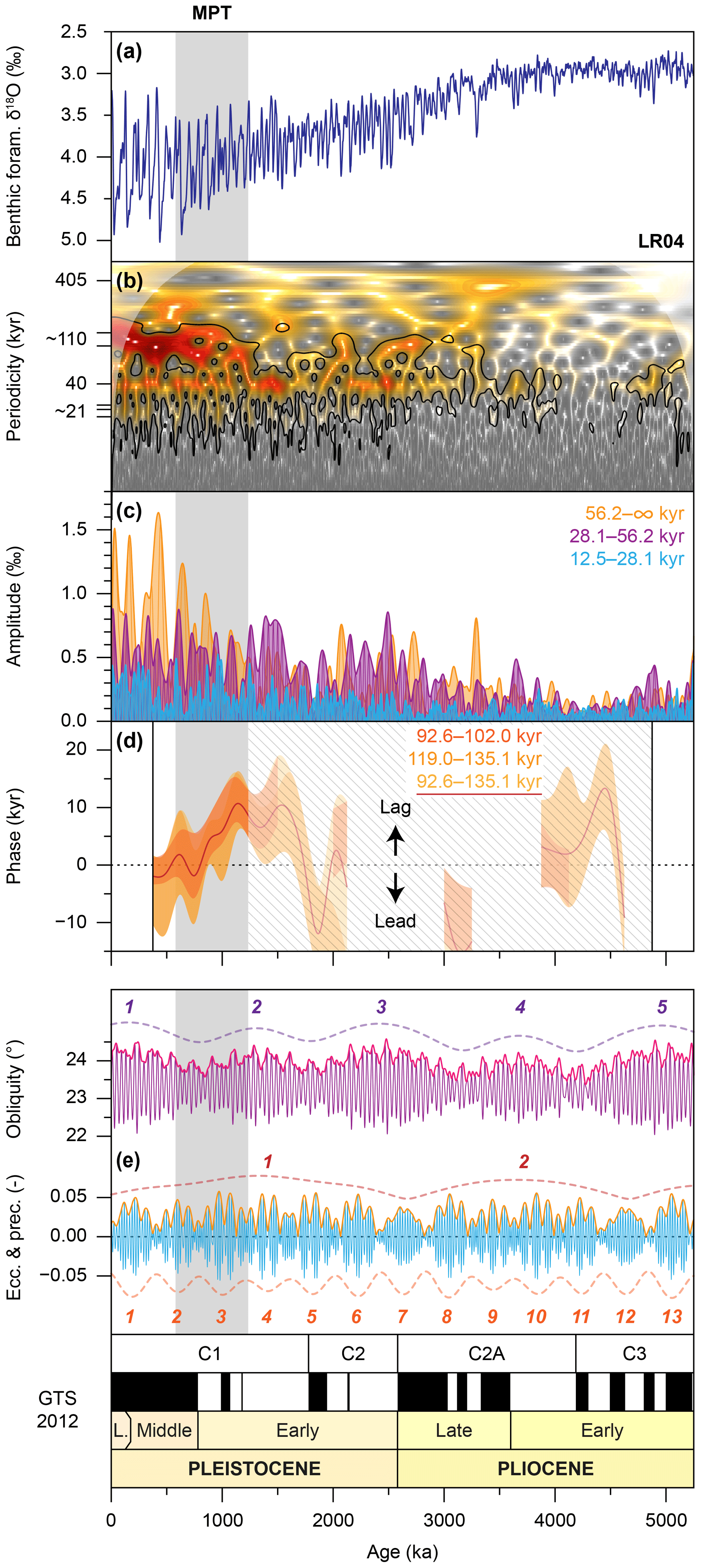
Figure 1Sinusoidal properties of Pliocene and Pleistocene climate cycles (after Lisiecki and Raymo, 2005a; Lisiecki, 2010). (a) Resampled LR04 benthic foraminiferal δ18O stack. (b) Wavelet analysis of the LR04 stack after detrending. Black contours represent 95 % significance. (c) Absolute amplitude modulations and filters of the ∼110, 40, and ∼21 kyr periodicities. (d) Phase evolution of the ∼110 kyr periodicity with respect to eccentricity (Laskar et al., 2011a, b), computed over a 750 kyr sliding window shown only when coherent (Paillard et al., 1996). (e) Astronomical and magnetostratigraphic reference records (Hilgen et al., 2012).
2.2 Quantifying geometries using central moments
Skewness and asymmetry are quantified using both the third central moment and bispectral methods (Figs. 2, S2, and S3 in the Supplement) (see Sect. 2.3.3 for bispectral method) (Elgar, 1987). Excess kurtosis is quantified using the fourth central moment only, because no trispectra were calculated (Fig. 2). Using third-moment quantities, skewness is determined by Eq. (1):
where the overbar indicates the mean value and where 〈〉 is the time-averaging operator (i.e. window length over which the computation is performed) (Doering and Bowen, 1995), and asymmetry is determined following Eq. (2):
where H is the Hilbert transform (Kennedy et al., 2000). Skewness is a measure for the dissymmetry of a cycle relatively to a horizontal axis (Fig. 2b), whereas asymmetry is a measure for the dissymmetry of a cycle through time (Fig. 2c). Using fourth-moment quantities, excess kurtosis is defined by Eq. (3):
Excess kurtosis is a measure for the flatness or peakedness of the extrema of a cycle. Cycles with flat tops and bottoms (i.e. platykurtic cycles), such as a square wave, have negative excess kurtosis values, whereas sharp-topped and sharp-bottomed cycles (i.e. leptokurtic cycles), such as a cardiogram, have positive kurtosis value (Fig. 2d).
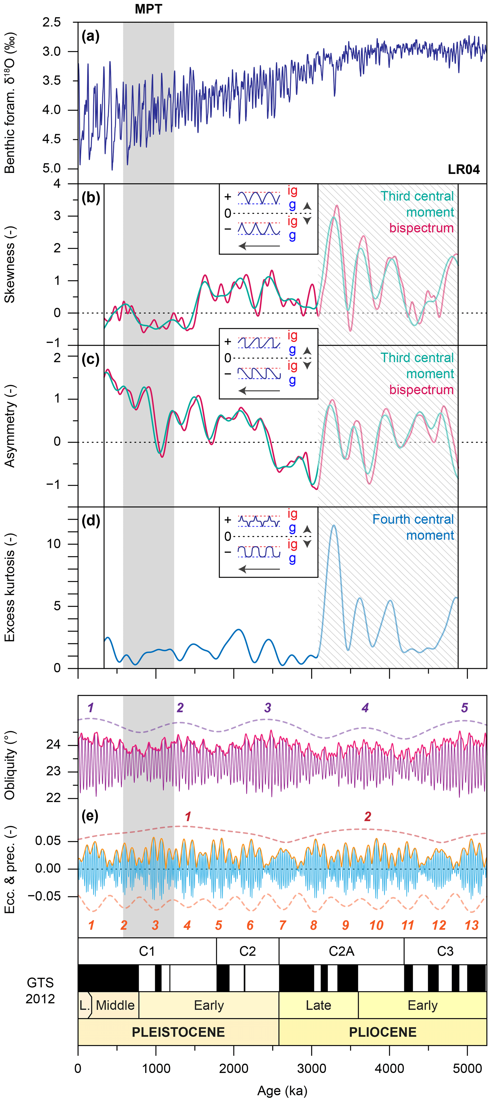
Figure 2Non-sinusoidal properties of Pliocene and Pleistocene climate cycles (after Lisiecki and Raymo, 2007). (a) As in Fig. 1. (b) Evolution of glacial–interglacial cycle skewness, (c) asymmetry, and (d) excess kurtosis (i.e. normalised third and fourth central moments), computed over a 668 kyr sliding window, using standard (teal and blue lines) and bispectral (pink lines) methods. Inset boxes show corresponding cycle shapes. The arrow shows the direction of time, “g” indicates glacial, and “ig” indicates interglacial. We focus the geometry interpretation on the time interval with the greater amplitude variability in the record (transparent area). (e) As in Fig. 1.
2.3 Bispectral analysis
2.3.1 The bispectrum
In contrast to spectral analysis (e.g. using the fast Fourier transform), which gives the distribution of variance of a sinusoidal signal with frequency, bispectral analysis describes the distribution of non-sinusoidality with frequency (King, 1996). The skewness of a cycle is described by the real part of the bispectrum, whereas the asymmetry of a cycle is deconvolved in the imaginary part of the bispectrum. The bispectrum shows nonconservative relative energy exchanges among frequencies of a single time series. Energy transfers in the bispectrum computed on the LR04 stack are expressed in ‰3 kyr2, which constitutes a statistical measure of energy. (We refer to Sect. 2.4.1 for an explanation of conservative net energy exchanges and Sect. 4.2 for a discussion of the scaling of conservative to absolute energy exchanges). Energy transfers can only occur, and be analysed by the bispectrum, if both the frequencies (f) and phases (Phi, φ, in radians) of these non-sinusoidal cycles are coupled: i.e. and , respectively (Hagelberg et al., 1991). Thus, for any possible combination of three frequencies, the bispectrum assesses whether there is a coupling, and if so, whether energy exchanges occur. The transfer of energy in these so-called triad interactions is nonlinear, because the changes in cycle amplitudes (A) do not sum and have a currently unknown, and probably variable, coupling through time (i.e. ; see Sect. 4.2). We note that the meaning of “cycle”, “frequency” and/or “periodicity” is different when referring to either the time or frequency domain. For example, a “single” cycle in a time series is often composed of multiple frequency components, which can be deconvolved by (bi)spectral analysis. However, for textual purposes, we use these words interchangeably, regardless of their reference to a specific domain.
The bispectrum is defined by Eq. (4):
where E[…] is the ensemble average of the triple product of complex Fourier coefficients C at the difference frequencies f1, f2, and their sumf3 (i.e. ), and the asterisk indicates complex conjugation (Hasselmann et al., 1963). In this study, we focus on the imaginary part of the bispectrum (hereafter often referred to as “bispectrum”, unless indicated otherwise), following studies on ocean waves (e.g. Herbers et al., 2000; de Bakker et al., 2015), because according to bispectral theory most energy transfers are associated with asymmetric cycle shapes (i.e. wave forms), and because the climate cycles of the Middle and Late Pleistocene have high amplitudes (Fig. 1) and are highly asymmetric (Fig. 2). Furthermore, conservative net energy exchanges between the coupled frequencies that are located in the imaginary part of the bispectrum can be computed if we assume a simple coupling coefficient between frequencies. Prior to bispectral analysis, we detrend the data and subsequently apply a tapering function using a Hann (a.k.a. Hanning) window that also mitigates spectral leakage (Hagelberg et al., 1991) and then multiply the data by an energy correction factor to adjust for the change in amplitude that results from the windowing.
2.3.2 Interpreting the bispectrum
The x and y axes in the bispectrum, which correspond to f1 and f2, respectively, are mirror images of each other and share a symmetry axis at x=y (Fig. 3) (Hasselmann et al., 1963). Therefore, only the positive, one-eighth part of the bispectrum is depicted, which is subdivided into 15 zones (see Sect. 2.4.2, Table A1). For triad interactions, only two outcomes exist: either two frequencies (by definition, f1 and f2) gain energy (though not necessarily in equal measures), and one frequency (i.e. f3) loses energy, or f1 and f2 lose energy (ditto), and f3 gains energy. Frequencies f1 and f2 are the so-called difference frequencies, while frequency f3 is referred to as a sum frequency. Frequencies often participate in multiple interactions, and depending on the interaction, they act as either a difference frequency or a sum frequency. A particular frequency can thus receive energy through one interaction and simultaneously lose energy in another interaction.
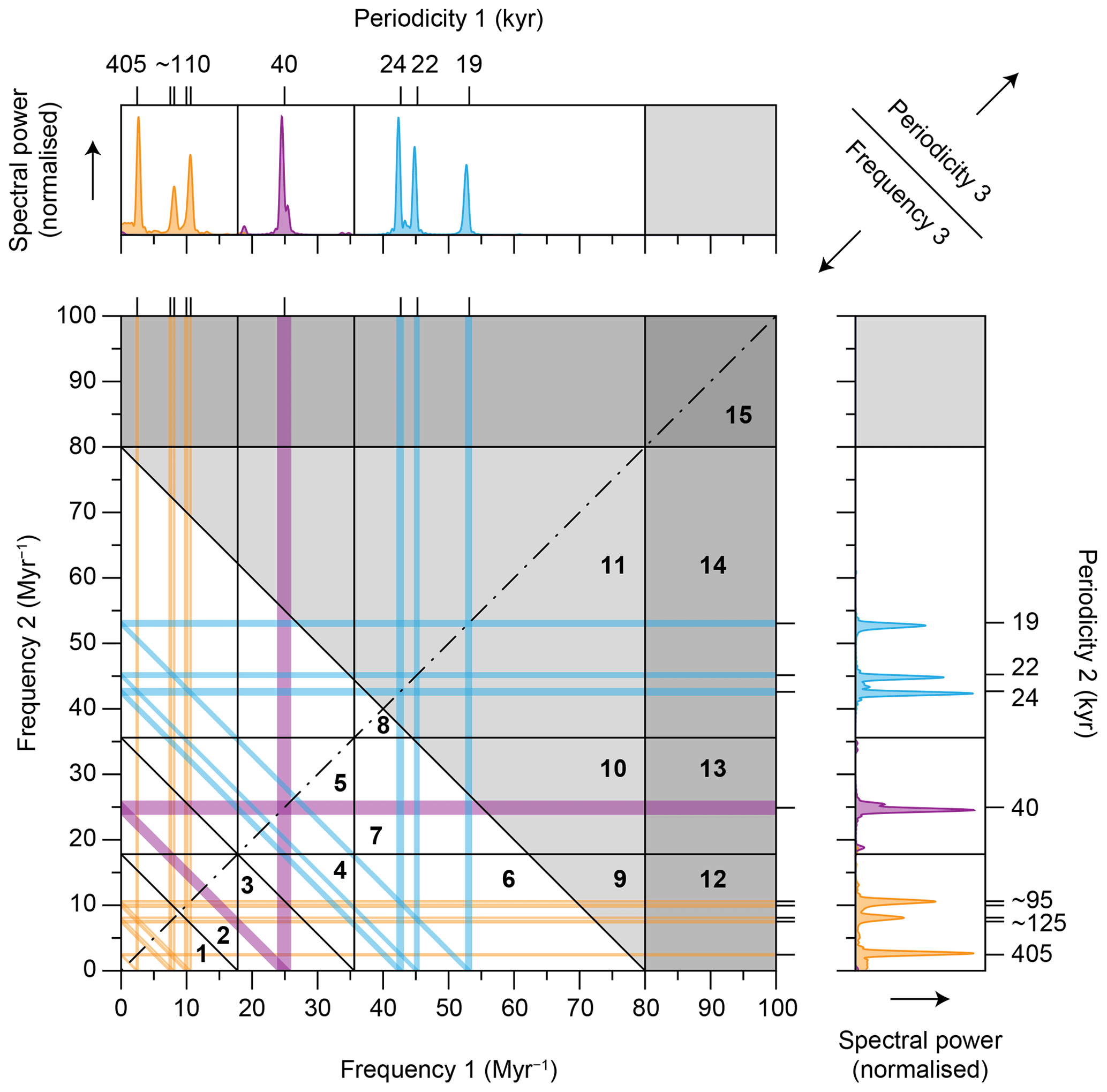
Figure 3Bispectral zonation scheme. Bispectra of climate cycles can be subdivided into 15 zones that reflect unique combinations of three frequency bandwidths. Orange, purple, and blue lines represent the main astronomical frequencies of the eccentricity, obliquity, and precession cycles, respectively (this colour coding is consistent throughout the paper). The grey shaded areas represent suborbital periodicities. Difference frequencies f1 and f2 are plotted along the along the horizontal and vertical axes, respectively. Sum frequencies f3 (i.e. f1+f2) are depicted as diagonal lines in the bispectrum. See also Table A1 for a list of bispectral zones and Table A2 for a list of triad types among the main astronomical frequencies in the bispectrum.
To help the interpretation of the bispectrum, we depict the main astronomical frequencies in the bispectrum with coloured lines (Fig. 3). Vertical and horizontal lines correspond to the difference frequencies (f1 and f2, respectively), and diagonal lines correspond to the sum frequency (f3). Junctions between lines highlight the locations in the bispectrum where interactions occur between three periodicities (i.e. triad interactions) of which at least one is an astronomically paced climate cycle, which can also interact with itself (Fig. 3; see also Table A2). No frequency axis is associated with sum frequency f3, but its value can be read off at the crossing points with the x and y axes of the bispectrum or by summing the x and y coordinates of the difference frequency axes at any point along the diagonals (Fig. 3).
We follow the convention and define a triad interaction as negative or positive if f3 either loses (blue colours) or gains (red colours) energy, respectively (Fig. 4). In written form, energy gains at a particular frequency are marked by an upward-pointing arrow (↑) and losses by a downward-pointing arrow (↓). Bispectral notation of triad interactions are given as Bf(f1, f2, f3) in the frequency domain (Myr−1) and as Bp(p1, p2, p3) in the periodicity domain (kyr). For palaeoclimatological purposes, we will mainly focus on the periodicities for which the corresponding frequencies can easily be looked up in Table A2. We refer to the relevant part of the bispectrum as “Re” (i.e. real) and “Im” (i.e. imaginary), which are given in superscript (BRe and BIm, respectively). Thus, if we consider a negative triad interaction, located in the imaginary part of the bispectrum, between p1, a 40 kyr obliquity-paced cycle (i.e. f1=25.0 Myr−1), and p2, a ∼95 kyr eccentricity-paced cycle (i.e. f2=10.5 Myr−1), that results in a loss of energy at p3, the ∼28 kyr periodicity (i.e. f3=35.5 Myr−1), this is given as (40↑, 95↑, 28↓) (i.e. (25.0↑, 10.5↑, 35.5↓)) (Fig. 4a).
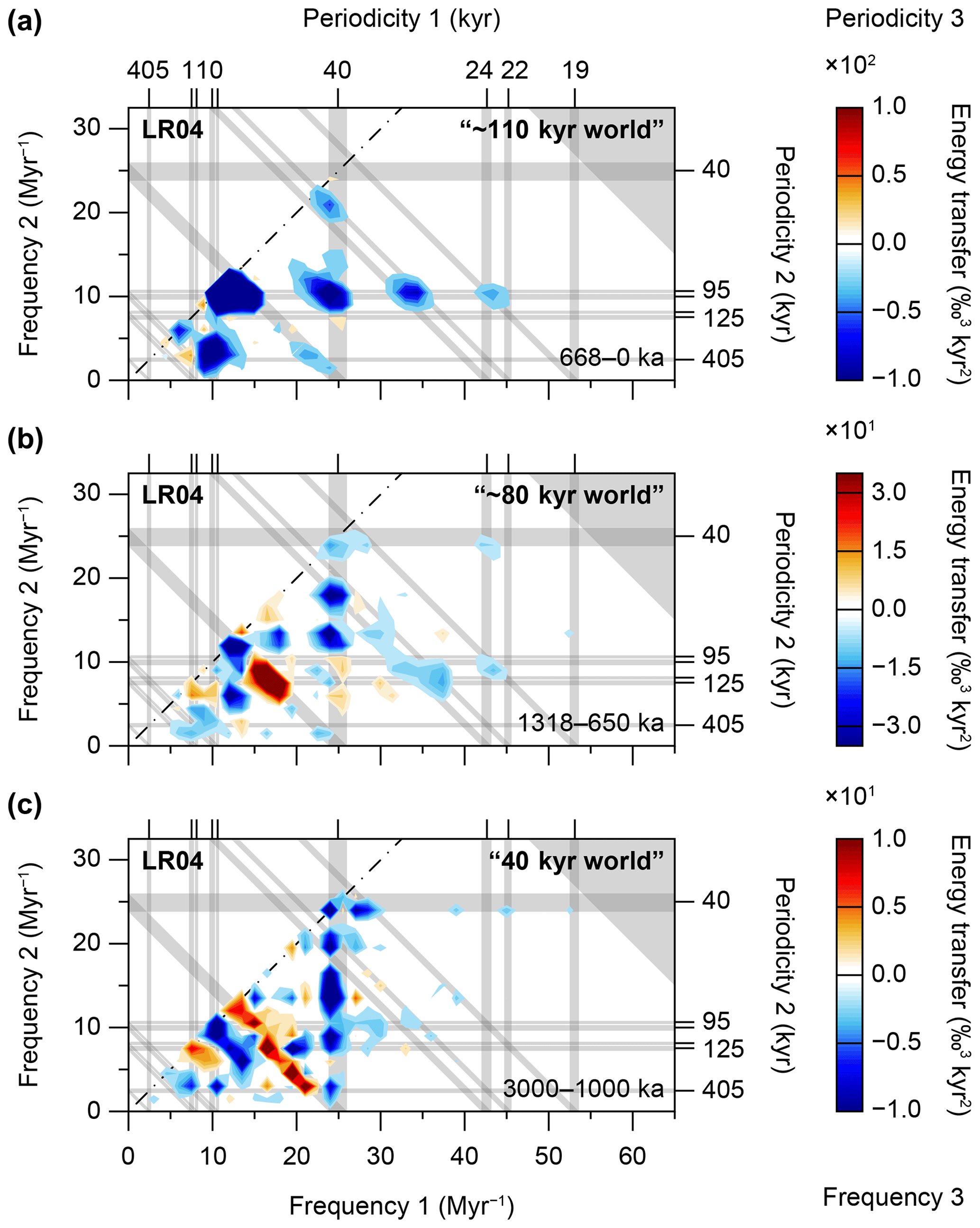
Figure 4Bispectra of Pliocene and Pleistocene climate cycles. (a) Imaginary part of a bispectrum of the Middle and Late Pleistocene “∼110 kyr world”. Age range =668 to 0 ka. Resampling resolution =1 kyr−1. Window length =668 kyr. Block length =668 kyr. Number of blocks =1. Number of merged frequencies =1. Frequency resolution =1.50 Myr−1. Degrees of freedom = 2. Min value = −598 ‰3 kyr2. Max value =51 ‰3 kyr2. (b) Imaginary part of a bispectrum of the mid-Pleistocene transition “∼80 kyr world”. Age range =1318 to 650 ka. Resampling resolution =1 kyr−1. Window length =668 kyr. Block length =668 kyr. Number of blocks =1. Number of merged frequencies =1. Frequency resolution =1.50 Myr−1. Degrees of freedom =2. Min value ‰3 kyr2. Max value =73 ‰3 kyr2. (c) Imaginary part of a bispectrum of the Pliocene and Early Pleistocene “40 kyr world”. Age range =3000 to 1000 ka. Resampling resolution =1 kyr−1. Window length =2000 kyr. Block length =2000 kyr. Number of blocks =1. Number of merged frequencies =3. Frequency resolution =1.50 Myr−1. Degrees of freedom =6. Min value ‰3 kyr2. Max value =23 ‰3 kyr2. Note the different scaling of the z axes between panels (a), (b), and (c). These bispectra are computed on the LR04 stack (see methods section) (Lisiecki and Raymo, 2005a).
We note that within this study, we almost exclusively focus on the imaginary part of the bispectrum. This approach contrasts with previous palaeoclimate investigations that used the bicoherence spectrum (see, e.g. Hagelberg et al., 1991; von Dobeneck and Schmieder, 1999; Wara et al., 2000; Huybers and Curry, 2006; Da Silva et al., 2018). In short, bicoherence is a measure of the coherency between the real and imaginary parts of the bispectrum (i.e. where both parts have strong interactions) and is marked by positive values only (see, e.g. Elgar and Sebert, 1989; de Bakker et al., 2014). Conversely, the real and imaginary parts of the bispectrum transform skewed and asymmetric cycle geometries into their composite frequency components, respectively, and both parts are characterised by positive as well as negative interactions.
2.3.3 Quantifying geometries using the bispectrum
Adopting the bispectral method to extract cycle geometries (Figs. 2, S2, and S3) (Elgar, 1987), skewness and asymmetry are computed from the biphase. The biphase reflects the ratio between the real and imaginary parts of the bispectrum. The biphase is defined by Eq. (5):
where n and l range from 1 to the Nyquist frequency N, with n > l and (Elgar, 1987), and fp refers to the primary frequency (a.k.a. natural or resonance frequency, or first harmonic). We note that positive asymmetry values correspond to a dominance of negative interactions (i.e. a loss of energy at f3) in the imaginary part of the bispectrum, and vice versa, negative values for this geometry are indicative of an overall dominance of positive interactions (i.e. a gain of energy at f3).
2.4 Power spectral density and net energy transfers
2.4.1 Integration of the spectrum and bispectrum
To quantify power spectral density, we apply a standard integration of the power spectrum. To obtain conservative net energy transfers per frequency (defined by the nonlinear source term Snl) and hence to extract the total gain or loss in energy per climate cycle over a specific time interval (i.e. window), we integrate over the imaginary part of the bispectrum and multiply it by a coupling coefficient. For palaeoclimate time series, no coupling coefficient has been determined previously. Therefore, we make minimum assumptions and use a coupling coefficient that only corrects for frequency . A comparable correction for frequency is also part of the Boussinesq scaling that is used for ocean waves (e.g. Herbers and Burton, 1997; Herbers et al., 2000). The correction for frequency () insures energy conservation during triad interactions, because more energy is exchanged among the higher frequencies. Furthermore, this correction allows for qualitative interpretations of conservative net energy exchanges across the spectrum. If a more appropriate coupling coefficient for palaeoclimatic purposes were to be deduced, it could also scale the conservative net energy transfers of the bispectrum (already corrected using Snl during integration) to absolute energy transfers that can be compared to (changes in) power spectral density (see Sect. 4.2). We express the integral of Snl in terms of an integration, or summation, over the positive quadrant of the bispectrum alone or equivalently in sum and difference interactions following Eq. (6):
where the sum contributions are expressed by Eq. (7):
and the difference contributions are expressed by Eq. (8):
The sum contributions are obtained by integrating diagonally over the bispectrum, and the difference contributions are obtained by integrating along vertical and horizontal lines, perpendicular to the x and y axes, respectively (Fig. 3). We track the evolution of net energy transfers through time by integrating over bispectra that are determined for consecutive and partially overlapping windows of the time series (i.e. a moving window) (Figs. 5, 6, and S3). Integration can be performed including all frequencies (i.e. over the entire imaginary part of the bispectrum) or over specific zones only, in the event that subsets of interactions need to be further examined (Fig. 3, Table A1) (de Bakker et al., 2015, 2016). After integration over the bispectrum, either totally or zonally, energy transfers computed on the LR04 stack are expressed in ‰3. Blue colours indicate a loss of energy at a specific frequency; red colours indicate a gain.
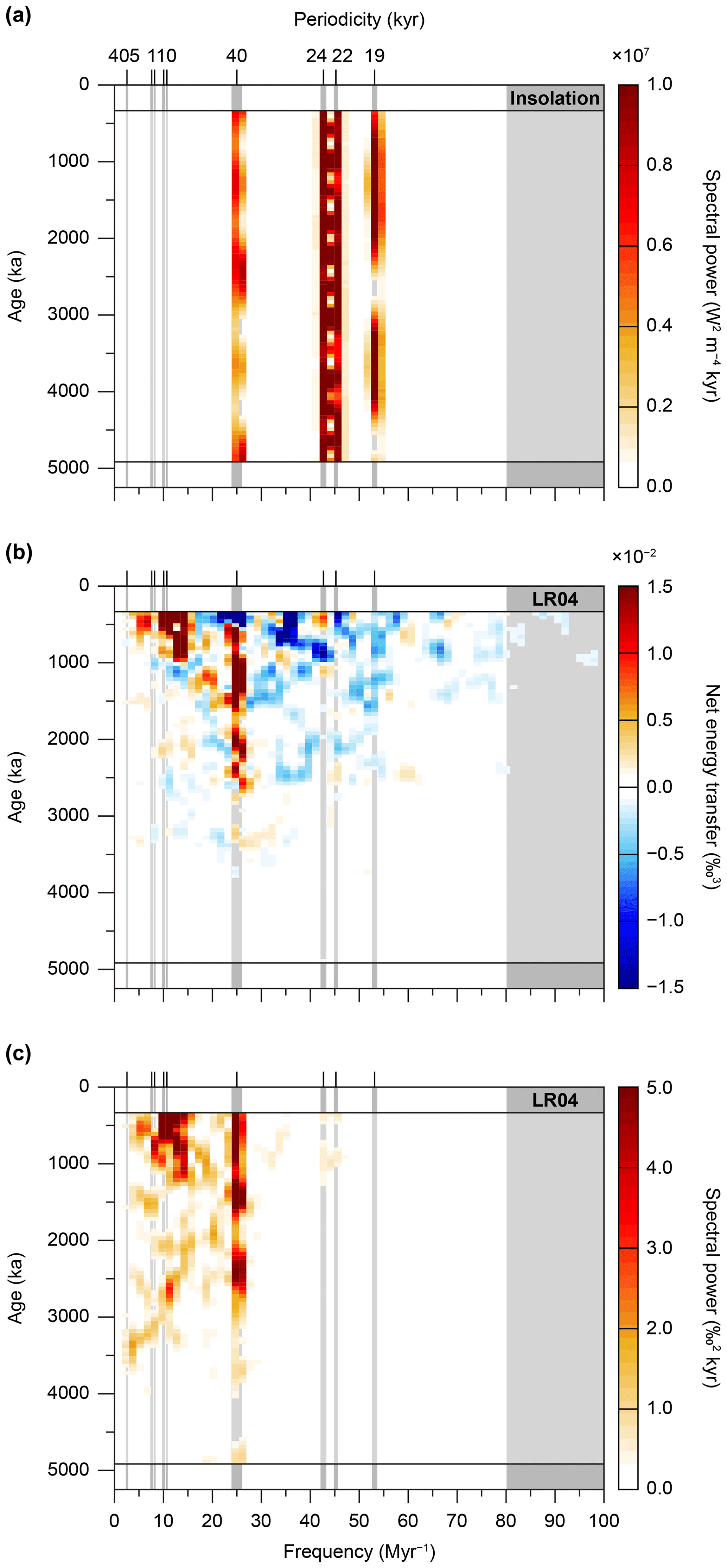
Figure 5(a) Input → (b) “black box” climate → (c) output. (a) Power spectral density of mean summer insolation (21 June to 21 September) at 65∘ N (Paillard et al., 1996; Laskar et al., 2004). (b) Conservative net energy transfers (i.e. after correction using the coupling coefficient) during the Pliocene and Pleistocene, computed by integrating over the entire imaginary part of the bispectrum (see methods section). Input data are the resampled LR04 stack (Lisiecki and Raymo, 2005a). (c) Power spectral density of the LR04 stack (Lisiecki and Raymo, 2005a). For all three panels, the window length is 668 data points (668 kyr), and the step size between partially overlapping windows is 50 data points (50 kyr). We used no blocks and did not merge frequencies. These settings yield a frequency resolution of 1.50 Myr−1 and 2 degrees of freedom.
2.4.2 Spectral and bispectral zones
To obtain more insight on the energy that is exchanged among eccentricity, obliquity, and precession cycles, we integrate the spectra and bispectra over separate zones (Fig. 3, Table A1). For bispectra, such a zonation approach was first applied in research concerned with nearshore ocean waves to distinguish between infragravity wave and sea-swell wave frequencies (de Bakker et al., 2015), and is adapted here to investigate the most important climate cycle bandwidths of the Pliocene and Pleistocene. The boundaries between the climate cycle zones are (arbitrarily) defined at frequencies of 17.8, 35.6, and 80.0 Myr−1 (i.e. periodicities of ∼56.2, ∼28.1, and 12.5 kyr). In total, 15 bispectral zones are defined (Fig. 3, Table A1), each of which represents a unique combination of three main groups of astronomically paced climate cycles and suborbital periodicities (i.e. supraorbital frequencies) that can interact and exchange energy with one other. We note that many periodicities without primary astronomical origin are included in these “eccentricity”, “obliquity”, and “precession” zones. We focus here on the results of the eight most important zones, namely those involving astronomically paced climate cycles (Figs. 7, 8, 9, S4, and S5). To better highlight the roles of all nonlinear interactions involving eccentricity, obliquity, or precession, we recombine (i.e. sum) the individual zones (Fig. 10).
3.1 Geometries of Pliocene and Pleistocene climate cycles
The geometry computations confirm the qualitative visual inspection of the LR04 globally averaged, benthic foraminiferal δ18O stack and show that strong non-sinusoidal cycle shapes are present in the data, especially during the Middle and Late Pleistocene parts of the record (Fig. 2) (Lisiecki and Raymo, 2007). We focus the geometry interpretations on the time interval with the greater amplitude variability in the δ18O record, which starts to increase (gradually) from ∼3000 ka onward. Between ∼3000 and ∼350 ka, the skewness of climate cycles varies between −0.5 and 1.0. Peak values of ∼1.0 are reached between ∼2500 and ∼1500 ka, after which skewness rapidly decreases at ∼1500 ka to negative values of −0.5 that slowly increase to 0.0 during the MPT (Fig. 2). Glacial–interglacial cycle asymmetry varies between about −0.5 and 1.5. The most prominent steps in asymmetry occur at ∼2500 and ∼1000 ka (the latter during the MPT) when values increase from about −0.5 to 0.5 and from approximately −0.2 to 1.2, respectively. These results compare well to those previously obtained on (stacks of) benthic foraminiferal δ18O records (Hagelberg et al., 1991; King, 1996; Lisiecki and Raymo, 2007). Excess kurtosis computations identify leptokurtic (thin-peaked) cycle shapes that vary between 0.5 and 3.0 from ∼3000 ka onward. Unlike skewness and asymmetry, which are marked by multi-Myr decreasing and increasing trends, respectively, no long-term trend can be discerned in Pleistocene cycle kurtosis (Fig. 2).
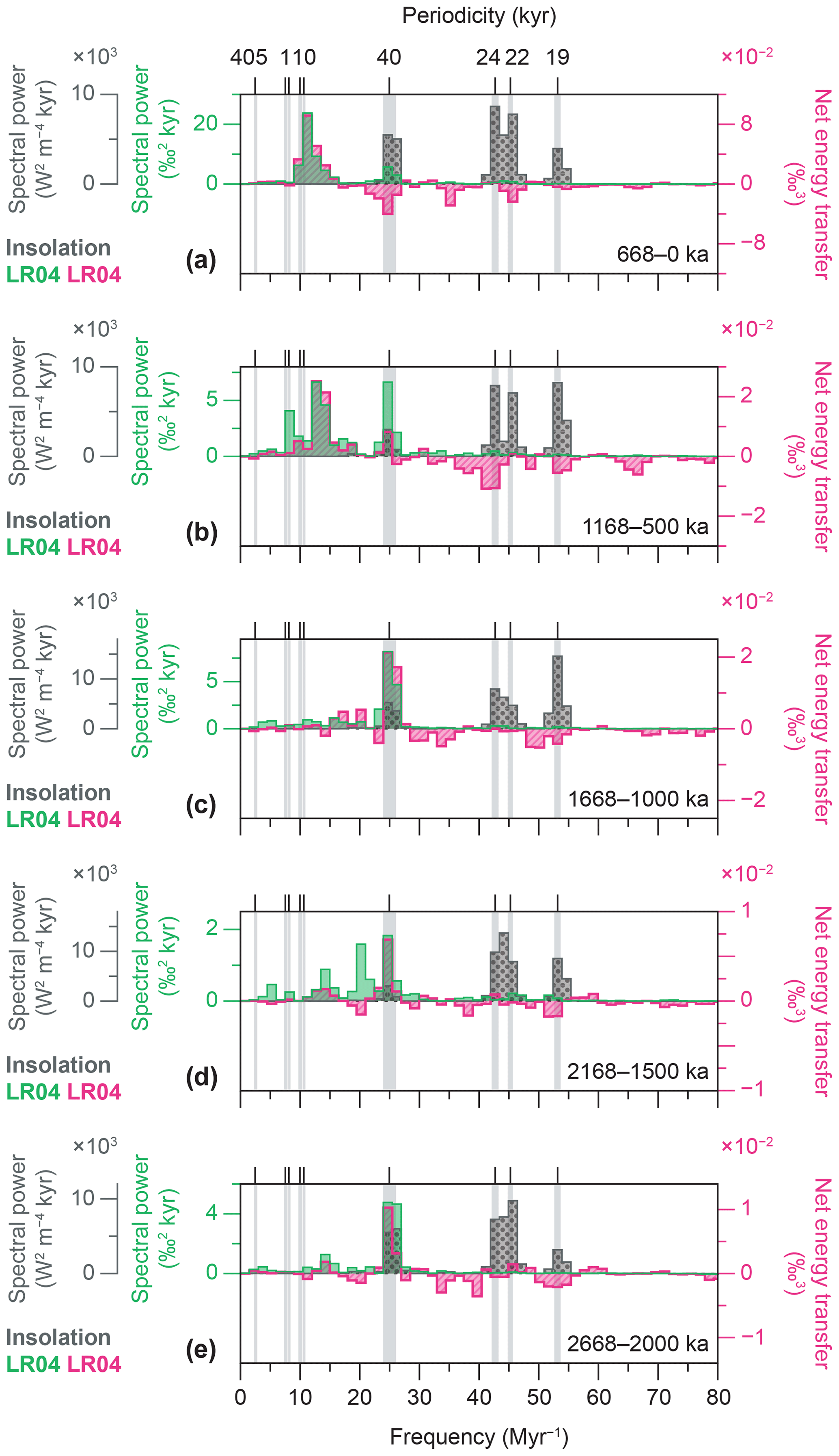
Figure 6Qualitative linkage of power spectra of insolation to those of climate via energy exchanges among climate cycles: (a) 334 ka, (b) 834 ka, (c) 1334 ka, (d) 1834 ka, and (e) 2334 ka. Computational settings are as in Fig. 5. Note that the scaling between the spectra and energy exchanges is arbitrary. Energy exchanges of the LR04 stack can be visually “scaled” (i.e. qualitatively compared) to the power spectrum of the LR04 by using multiplication factors of 430, 250, 360, 230, and 250 for panels (a) to (e), respectively.
3.2 Bispectra of Pliocene and Pleistocene climate cycles
Non-sinusoidal cycle shapes may indicate the potential for obtaining more information about nonlinear interactions among frequencies using higher-order spectral analysis (Hagelberg et al., 1991; King, 1996). We present three examples of Pliocene and Pleistocene bispectra (i.e. their imaginary parts), based on the LR04 stack, which are characterised by clear triad interactions (Fig. 4; see also Sect. 2.3.2.). The first example is a bispectrum across the Middle to Late Pleistocene (i.e. the “∼110 kyr world”), which shows clear and punctuated triad interactions concentrated where p2 equals 95 kyr (Fig. 4a). The main interactions are located at the following triads or their connecting lines: at (95↑, 405↑, 77↓), weakly at (95↑, 125↑, 54↓), from (95↑, 95↑, 48↓) via (69↑, 95↑, 40↓) to (80↑, 80↑, 40↓), broadly around (40↑, 95↑, 28↓), at (40↑, 51↑, 22↓), from (31↑, 95↑, 24↓) to (29↑, 95↑, 22↓), and weakly (but still visible) at the triple junction (24↑, 95↑, 19↓). Interactions at these triads (Table A2) are all negative, indicating that energy is mainly transferred to the 95 kyr (and 125 kyr) cycle from the three precession periodicities, the ∼28 kyr periodicity, and the 40 kyr obliquity periodicity. A very weak positive interaction is located at (125↓, 405↓, 95↑). Strong energy gains at the ∼110 kyr periodicity of eccentricity-modulated precession thus characterise the bispectrum of the Middle to Late Pleistocene interval.
The second example is a bispectrum across the mid-Pleistocene transition (i.e. the “∼80 kyr world”) and shows several negative interactions where either p1 or p2 is equal to ∼80 kyr (Fig. 4b). Particularly strong negative interactions are located at (80↑, 200↑, 57↓), (80↑, 80↑, 40↓), and (40↑, 80↑, 27↓). Also, (40↑, 58↑, 24↓) is strongly negative. We document one major positive interaction at (69↓, 95↓, 40↑), which connects to (59↓, 125↓, 40↑). Due to the relatively loosely distributed triad interactions in this bispectrum (Fig. 4b), compared to, for example, the bispectrum of the Late Pliocene to Early Pleistocene (Fig. 4c), it is more difficult to interpret dominant energy gains and losses directly from the bispectrum of the MPT. However, we observe an overall gain of energy at the 70 to 80 kyr periodicities, and a dual role for the 40 kyr periodicity, which operates as both the energy receiver and supplier simultaneously. We note that the ∼80 kyr periodicity is not an obvious triad of the primary astronomical cycles (Table A2), apart from the junction at (95↑, 405↑, 77↓), where no strong interaction is documented in this particular bispectrum. The 80 kyr periodicity thus starts as a “lower” harmonic or “subharmonic” (i.e. where “lower” and “sub” refer to the frequency domain) of the 40 kyr periodicity, which in turn is a first harmonic of obliquity forcing, as well as a “combination tone” of precession and non-astronomical periodicities (Table A2) (Pestiaux et al., 1988). This subharmonic origin for the 80 kyr periodicity is supported by the strong negative interaction at (80↑, 80↑, 40↓).
The third example is a bispectrum across the Late Pliocene to Early Pleistocene interval (i.e. the “40 kyr world”), which depicts negative and positive interactions, where both difference frequencies f1 and f2, and sum frequency f3 are equal to 25 Myr−1 (i.e. 40 kyr), respectively (Fig. 4c). More specifically, negative interactions are concentrated at and between triads along the lines from (40↑, 405↑, 36↓) to (40↑, 40↑, 20↓), and from (40↑, 40↑, 20↓) to (36↑, 40↑, 19↓), indicating a gain at the 40 kyr periodicity. Most notable is the strong negative interaction at (40↑, 93↑, 28↓) to (40↑, 83↑, 27↓). Other bispectral coordinates marked by negative interactions are those between (95↑, 95↑, 48↓) and (70↑, 150↑, 48↓). Positive interactions are concentrated on the line between the bispectral coordinates (80↓, 80↓, 40↑) and (44↓, 405↓, 40↑), which also indicate a gain at the 40 kyr periodicity by transfers from numerous other frequencies. Overall, the Late Pliocene to Early Pleistocene bispectrum depicts strong energy gains at the obliquity-paced 40 kyr periodicity through many triad interactions, some of which are with other astronomically paced climate cycles.
3.3 Qualitative comparison of summer-half insolation to the climate–cryosphere proxy record
Figure 5 shows three time-evolutive spectral and bispectral analyses for the Pliocene–Pleistocene time interval. It compares the total power spectral density of summer-half insolation at 65∘ N (Fig. 5a) (Laskar et al., 2004) to the total energy transfers and total power spectral density of the LR04 benthic foraminiferal δ18O stack (Fig. 5b and c, respectively). This insolation curve constitutes a classical shorthand for the complex external forcing of the ice ages (not shown, but see Figs. 1e and 2e for individual records of precession, obliquity and eccentricity) (Köppen and Wegener, 1924; Milankovitch, 1941). Figure 6 highlights five equally spaced (500 kyr apart) time slices of the three panels of Fig. 5. Figure 7 depicts three zonally averaged frequency slices of the three panels of Fig. 5, namely the “eccentricity”, “obliquity”, and “precession” zones (see Sect. 2.4.2.), as well as the total of all frequencies combined.
3.3.1 Power spectral density of insolation
The time-evolutive power spectra of insolation are marked by high spectral power at the precession and obliquity periodicities, and the near absence of spectral power at the eccentricity periodicities (Figs. 5a, 6, and 7a) (Hays et al., 1976; Berger, 1977). Furthermore, it is characterised by amplitude variability in spectral power at these periodicities, which is governed by the long-term (eccentricity) modulations of obliquity and precession. These amplitude modulations have durations of ∼180 kyr (not detected here due to window length) and 1.2, 2.4, and 4.8 Myr for obliquity, and 405 kyr and 2.4 Myr for eccentricity-modulated precession (Figs. 5a and 7a). Concurrent with the MPT, we document the sharpest decrease in total spectral power of the entire Pliocene and Pleistocene, which is largely due to a decrease in precession power from maximum values (Fig. 7a) (Laskar et al., 2004). This is indicative of a reduction in the perturbation of the Earth's system that results from a smaller difference in insolation forcing between the hemispheres (i.e. reduced seasonality).
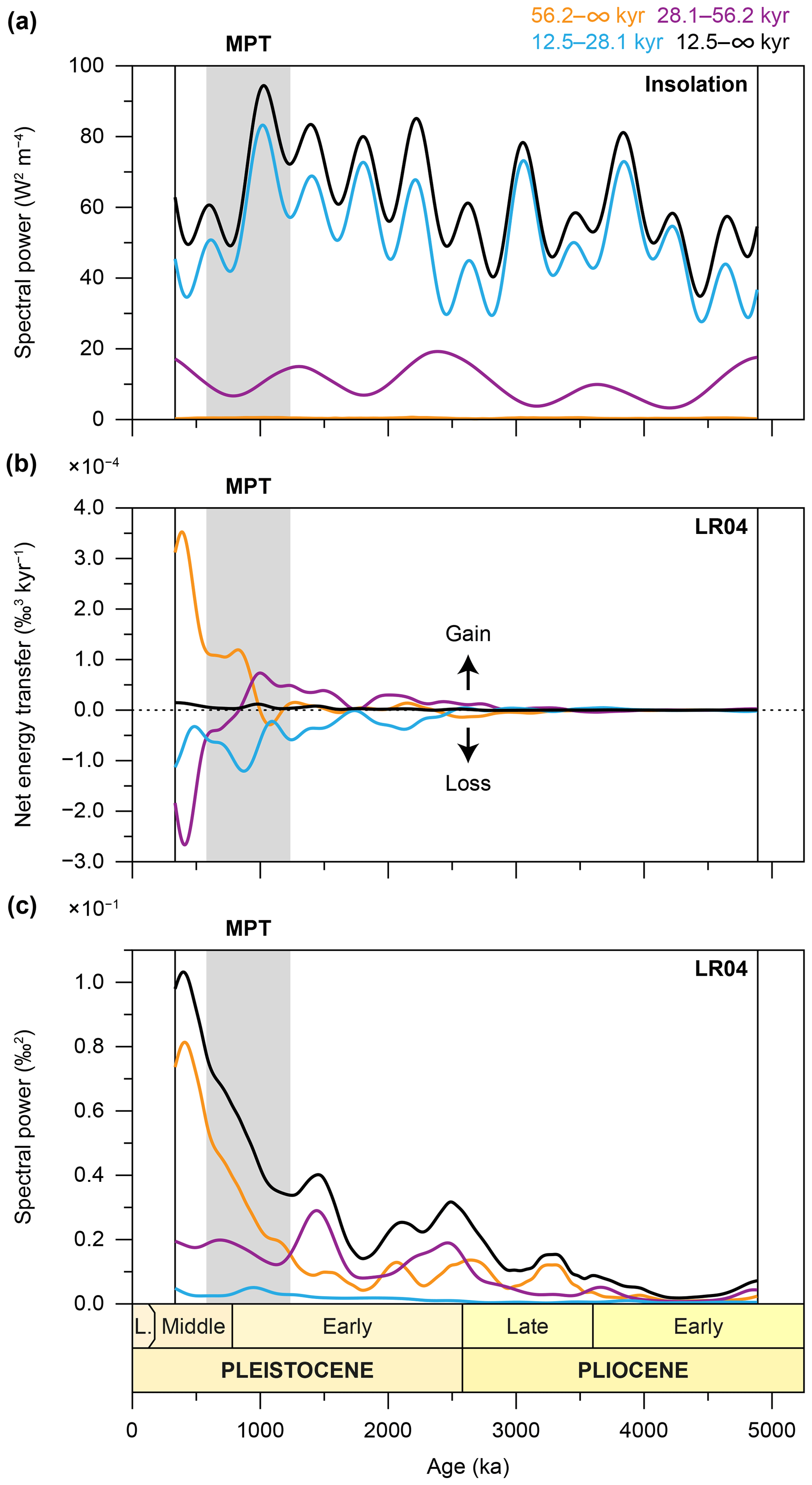
Figure 7Integration of the spectra and bispectra per astronomical bandwidth (top right). (a) Totally and zonally integrated spectra of mean summer insolation (21 June to 21 September) at 65∘ N. (b) Totally and zonally integrated bispectra of the LR04 stack. (c) Totally and zonally integrated spectra of the LR04 stack. Computational settings are as in Fig. 5.
3.3.2 Energy transfers among climate cycles
Figures 5b and S3 depict the conservative net energy transfers among (astronomically forced) climate cycles as present in the LR04 stack. The net energy transfers show how energy is redistributed over the power spectrum among astronomically paced and non-astronomically paced climate cycles. They reveal strong increases in both energy gains (in red) and losses (in blue) toward the present, and from ∼1000 ka onward several consecutive shifts in energy transfers from lower to higher periodicities occur (Fig. 5b). Energy gains are highly concentrated at the 40 kyr periodicity from ∼2500 ka onward and are marked by a modest 1.2 Myr beat in amplitude (Figs. 5b and 7b). A second location of strong energy gains is the ∼80 kyr periodicity from ∼1000 ka onward (Fig. 6b), which at ∼700 ka shifts (Fig. 5b) to a dominant gain for the 95 kyr component (Fig. 6a). Further energy gains are located at a ∼200 kyr periodicity from ∼750 ka onward, a 50 to 60 kyr periodicity between ∼1500 and 500 ka, and (very weak) at the 24 kyr periodicity from ∼650 ka onward (Fig. 5b). Energy losses are also observed in the total integration over the bispectra (Figs. 5b, 6, and 7b). However, these losses are generally of smaller amplitude per cycle and are distributed across a greater number of periodicities, in comparison to the highly concentrated energy gains (Figs. 5b and 6). Despite this more dispersed pattern of energy losses, we highlight the more conspicuous decreases: the 40 kyr periodicity from ∼550 ka onward, the 30 to 36 kyr periodicities between 1500 and 1000 ka, the 30 to 26 kyr periodicities between ∼2500 and ∼2000 ka, the ∼28 kyr periodicity from ∼800 ka onward, the 24 kyr periodicity between ∼1000 and ∼800 ka, the 22 kyr periodicity from ∼700 onward, the 19 kyr periodicity from 2000 ka onward, and the 15 kyr periodicity intermittently from ∼1000 ka onward (Fig. 5b).
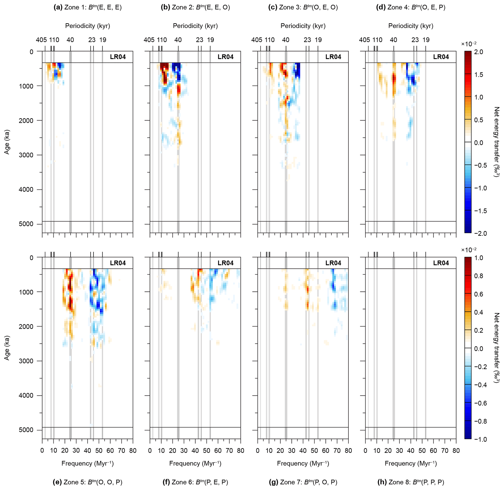
Figure 8Disentangling “black box” climate. Conservative net energy transfers during the Pliocene and Pleistocene over specific zones in the imaginary part of the bispectrum (see methods section). Computational settings are as in Fig. 5b. (a) Zone 1. (b) Zone 2. (c) Zone 3. (d) Zone 4. (e) Zone 5. (f) Zone 6. (g) Zone 7. (h) Zone 8. See also Fig. 3 and Table A1.
3.3.3 Power spectral density of climate cycles
Time-evolutive power spectral analysis of the LR04 record is characterised by high-amplitude variability at the 40 kyr obliquity-paced cycle, from approximately 4000 ka onward (Figs. 5c, 6, and 7c). In addition, distinct ∼80 and ∼110 kyr cycles of rapidly increasing amplitude are documented from ∼1200 ka onward, marking the MPT (Fig. 6b) and post-MPT (Fig. 6a) intervals, respectively (Lisiecki and Raymo, 2005a, 2007). We note that the 125 kyr component of the ∼110 kyr signal in the power spectra (Fig. 5c) is not present in the integration over the bispectrum (Fig. 5b) A relatively weak ∼200 kyr cycle is present from ∼750 ka onward (Fig. 5c). No strong precession response is present (Raymo and Nisancioglu, 2003; Raymo et al., 2006). The 40 kyr cycle in δ18O partially mimics the 1.2 Myr amplitude modulation of the obliquity cycle, especially from ∼3000 ka onward (Fig. 5c) (Lourens and Hilgen, 1997; Lisiecki and Raymo, 2007). We draw attention to a subtle “arc” in spectral power (absent in bispectral power), which starts with a strong 405 kyr cycle, at ∼3500 ka, that becomes gradually shorter in duration until it resonates with the 95 kyr eccentricity modulation of precession, at ∼2650 ka, and then culminates in several weaker 70 to 80 kyr cycles at ∼2000 ka (Fig. 5c; see also Fig. 1b) (Lisiecki, 2010; Meyers and Hinnov, 2010; Viaggi, 2018).
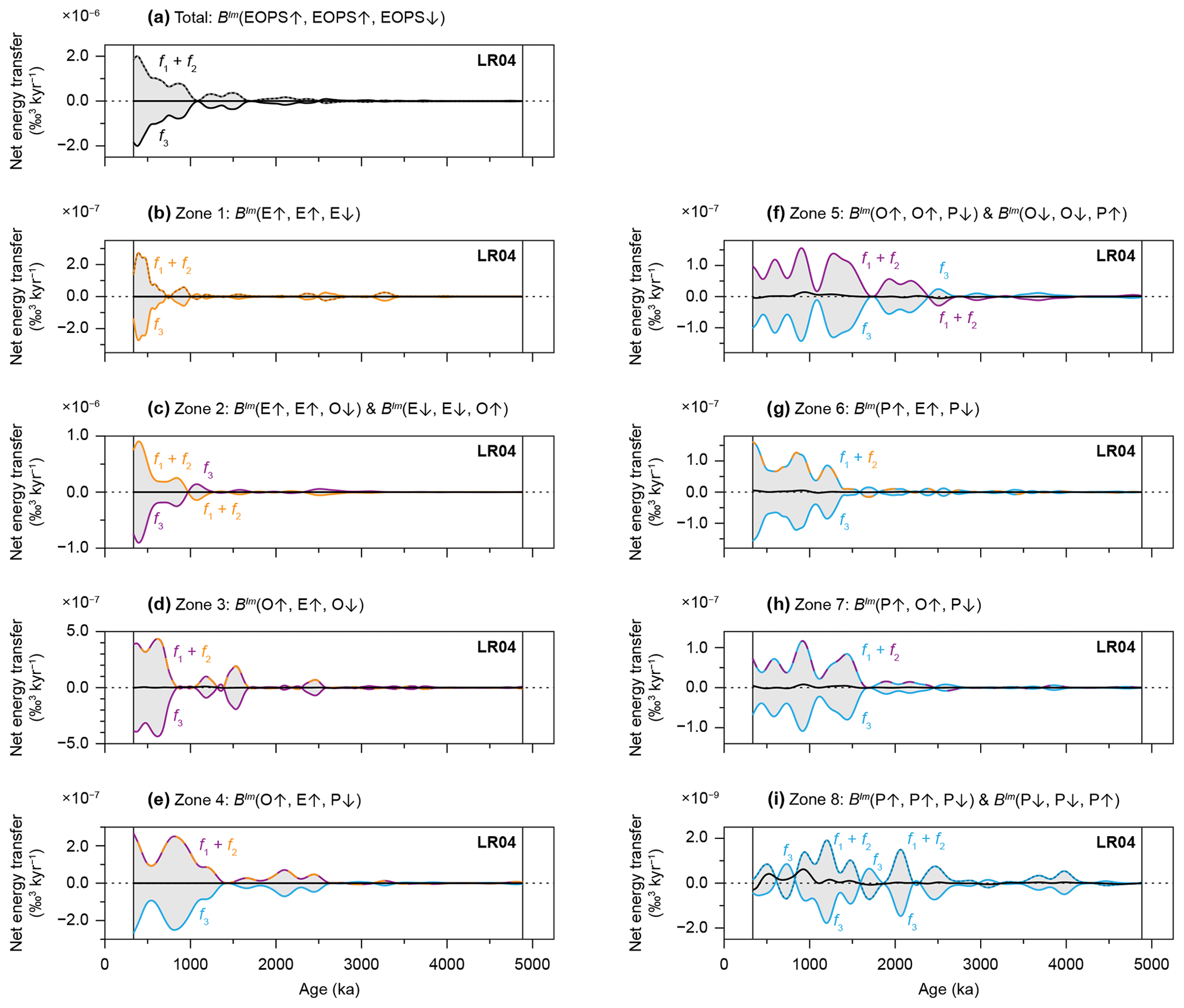
Figure 9Conservation of energy in triad interactions located in the imaginary part of Pliocene and Pleistocene bispectra. Conservativity of (a) the entire bispectrum (Fig. 5b) and (b) Zone 1, (c) Zone 2, (d) Zone 3, (e) Zone 4, (f) Zone 5, (g) Zone 6, (h) Zone 7, and (i) Zone 8, of the bispectrum (Fig. 8). Energy gains or losses of f1 and f2 (dashed lines) are computed using Eq. (8), those of f3 (single coloured lines) following Eq. (7), and their differences (black lines) by Eq. (6).
3.4 Zooming in on energy transfers
To better understand the different roles of specific (bandwidths of) climate cycles in nonlinear interactions, we determine conservative net energy transfers per bispectral zone (Figs. 8, S4, and S5). These zones reflect the “layers” that make up total energy exchanges as depicted in Fig. 5b. We assess if triad interactions are conservative of energy for each of the bispectral zones and for the entire bispectrum (Fig. 9). Lastly, we recombine the bispectral zones again for frequency bandwidths involving precession-, obliquity-, or eccentricity-paced climate cycles to highlight their influences in nonlinear interactions (Fig. 10).
3.4.1 Zonal energy transfers
In Zone 1, from 1000 ka onward, we document a modest exchange of energy between the (eccentricity-related) periodicities in the range from ∼200 to 50 kyr (Fig. 8a). Notably, from ∼500 ka onward, periodicities of ∼80 to 50 kyr predominantly lose power, whereas those between ∼200 and ∼80 kyr mainly gain energy. Stronger exchanges are documented in Zone 2 (Fig. 8b). Especially the 40 kyr obliquity-paced cycle gains energy between 3500 and 900 ka in this zone, after which it loses energy from 900 ka onward. Also, the 50 to 60 kyr periodicity loses energy, especially from ∼600 ka onward. Between ∼1100 and ∼800 ka, a single periodicity of ∼87 kyr gains power. At ∼750 ka, this periodicity splits into an ∼80 kyr periodicity and a 95 kyr eccentricity-paced cycle, which both gain energy. In general, interactions in Zone 2 change from (weakly) positive (BIm(E↓, E↓, O↑)) to negative (BIm(E↑, E↑, O↓)) during the MPT (∼1000 ka), indicative of a change from escalating energy to higher frequencies, to a cascading from higher frequencies. We note that the energy exchanged through BIm(E, E, O) interactions (Zone 2) is almost of equal amplitude to that of all other interactions combined. Zones 3 to 5 are mainly marked by increases in energy at the 40 kyr cycle, roughly from 2500 ka onward (Fig. 8c to e). A smaller gain is documented in these zones (especially in Zone 3) at periodicities between ∼70 and 50 kyr from ∼1300 ka onward, and in Zone 3 at the 95 kyr cycle from ∼650 ka onward. Furthermore, we document decreases in energy at the ∼30 to 27 kyr periodicities, the ∼28 to 22 kyr periodicities, and the main precession periodicities of 24, 22, and 19 kyr, for Zones 3, 4, and 5, respectively. The switchover during the MPT, at about 750 ka, of energy loss at the 24 kyr cycle to a loss at the ∼28 kyr periodicity is associated with BIm(O, E, P) interactions (Zone 4) only. Zones 6 and 7 show weaker energy exchanges among the main astronomical periodicities. In Zone 6, the ∼27 and 24 kyr cycles show a small gain between ∼1000 and 700 ka, and from ∼700 ka onward, respectively. We document only very minimal direct fuelling of eccentricity-paced climate cycles by precession-paced climate cycles in this zone. Energy is lost in Zone 6 from 1500 ka onward at the 19 kyr cycle. In Zone 7, relatively weak gains are present at the main obliquity and precession cycles from 1500 ka onward. Energy losses of Zone 7 are located mainly at sub-precession periodicities of ∼15 to < 13 kyr (Fig. 8f and g). No energy exchanges of similar magnitude are documented in Zone 8 (Fig. 8h).

Figure 10Summed zonal integrations of the imaginary part of Pliocene and Pleistocene bispectra. Net energy transfers are computed by (a) summing Zones 1, 2, 3, 4, and 6 for triad interactions corresponding to the “eccentricity” bandwidth, (b) summing Zones 2, 3, 4, 5, and 7 for triad interactions corresponding to the “obliquity” bandwidth, and (c) summing Zones 4, 5, 6, 7, and 8 for triad interactions corresponding to the “precession” bandwidth. Panel (d) shows the corresponding summed zonal conservation of energy, with eccentricity in orange, obliquity in purple, and precession in blue.
Overall, the zonal integrations are marked by negative triad interactions and thus reveal a cascade of energy from the (sub)precession bandwidth to the obliquity and (ultimately) eccentricity bandwidths through several successive interactions (Fig. 8). These analyses further show that many periodicities fulfil a dual role that often remains stable through time, namely they serve simultaneously and persistently as energy provider and receiver. For example, the 24 kyr precession-paced cycle gains energy through BIm(P, E, P) and BIm(P, O, P) interactions, as documented in Zones 6 and 7, meanwhile losing energy through BIm(O, O, P) and BIm(O, E, P) interactions, as can be observed in Zones 4 and 5. As an exception to this persistent behaviour of many lower periodicities in transferring energy to higher periodicities, the role of the 40 kyr obliquity-paced cycle evolves but only in BIm(E, E, O) interactions (Zone 2). In Zones 3, 4, 5, and 7, the 40 kyr obliquity-paced climate cycle (predominantly) partakes in triad interactions as a difference frequency, and it continuously receives energy, mainly from precession. However, during the MPT (from ∼900 ka onward) in Zone 2, when the 40 kyr periodicity partakes in interactions solely as a sum frequency (f3) of two eccentricity components (f1+f2), it starts providing energy to the eccentricity bandwidth. The net (i.e. total) result of these opposing roles for the 40 kyr obliquity-paced cycle after the MPT is that energy losses overtake the gains (Figs. 5b and S3). However, the initial decrease of the integrated “obliquity” zone, between ∼1000 and 600 ka, is linked to the ∼28 kyr periodicity, not the 40 kyr periodicity (Fig. 5b).
3.4.2 Energy conservation
Computations of energy conservation, hereafter also referred to as “conservativity”, indicate that both the total as well as the zonal energy gains in triad interactions are commensurate with losses, given our assumed coupling coefficient (Fig. 9). The dominance of negative interactions (i.e. positive values for f1+f2 and negative values for f3) is indicative of a transfer within the Earth's climate–cryosphere system of insolation energy to lower frequencies. Energy is not well conserved in triad interactions documented by Zone 8. This is probably the result of the low number of interactions located in Zone 8 (Fig. 4) and the small area of this zone (Fig. 3).
3.4.3 Energy exchanges involving precession-, obliquity-, or eccentricity-paced climate cycles
To highlight the separate roles of the precession, obliquity, and eccentricity bandwidths during nonlinear interactions within the climate–cryosphere system, we recombine (i.e. sum) their respective bispectral zones of Fig. 8. To do so, we include those zones that contain either one, two, or three frequency components of a particular bandwidth (Figs. 3 and 10). The general pattern of an energy cascade is robust, but it becomes clearer that precession cycles do not contribute much to the fuelling of eccentricity-paced climate variability directly (Fig. 10a–c). The 40 kyr periodicity during the Middle and Late Pleistocene gains energy from precession-dominated interactions but loses energy in obliquity- and eccentricity-dominated interactions (Fig. 10a–c). A comparison of conservativity of the recombined zones that include at least one precession, obliquity, or eccentricity component indicates that approximately similar amounts of energy are exchanged in (triad) interactions involving obliquity as in those involving eccentricity (Fig. 10d).
4.1 Limitations
4.1.1 Age uncertainty and signal-to-noise ratio
By combining more than 50 individual benthic foraminiferal δ18O records, the LR04 stack simultaneously decreases the age uncertainty and increases the ratio of signal-to-noise considerably in comparison to any record individually (Lisiecki and Raymo, 2005a). Reduced age uncertainties and improved signal-to-noise ratios of stacked records may be obtained through the computation of averaged sedimentation rates in combination with statistical “binning” (Lisiecki and Raymo, 2005a), a probabilistic approach using a hidden Markov model (Ahn et al., 2017) or, as is the case in this reanalysis of the (1 kyr resampled/binned) LR04 stack, by additional statistical “smoothing” (Chaudhuri and Marron, 1999). For successful application of advanced bispectral analysis techniques, good age control and (very) high signal-to-noise ratios are needed, because the distributions of only small amounts of signal over time and frequency are considered (Hasselmann et al., 1963; King, 1996). For consecutive computational steps that use bispectra (i.e. the bispectrum and the integration over the bispectrum), increasingly better constrained and more noise-free data are required, because each step zooms in further on these small amounts of signal that are associated with non-sinusoidal geometries. The bispectra of climate cycles presented here show clear interactions (Fig. 4), and the integrations of the bispectrum reveal qualitatively consistent patterns of energy transfers for analysis with varying window lengths (Figs. 5b and S3). Therefore, we argue that the LR04 stack has sufficiently accurate age calibrations and a high enough signal-to-noise ratio for the successful application of advanced bispectral analysis.
4.1.2 Resolvability in time and frequency domains
Similar to the power spectrum, the bispectrum is marked by a trade-off between resolution in the time versus frequency domains (Fig. S3). Bispectral results become more significant, and can yield greater degrees of freedom, if a larger number of similarly shaped cycles, or waveforms, can be included for analysis (i.e. a lengthening of the window). For example, studies on natural nearshore waves or those on flume-generated waves (periodicities of seconds to minutes) use hour-long stable time series with high sampling resolutions and wave numbers (de Bakker et al., 2014). Bispectral analyses of such data sets are well resolved in the frequency domain. Furthermore, they permit the computation of robust confidence levels on the results and the selection of statistical settings that yield high degrees of freedom (e.g. Elgar and Guza, 1985; de Bakker et al., 2015). However, for the Pliocene and Pleistocene record, similar statistical objectives are unattainable, because no two climate cycles are alike and because of the low number of ∼110 kyr cycles in the Pleistocene (King, 1996; Lisiecki, 2010). As a result of this absence of “ergodicity” (i.e. a stable waveform through space and time), which characterises the unique Pliocene–Pleistocene climatic evolution as captured by the LR04 stack, relatively short window lengths are preferred to obtain well-resolved results in the time domain. The Hann windowing function visually clarifies the interactions in both the bispectra as well as the integrations over the bispectrum. Similarly to previous bispectral studies on the palaeoclimate archive (Hagelberg et al., 1991; King, 1996), we cannot define confidence levels for the bispectral analysis of the LR04 stack, because the number of cycles per window is too small. However, the bispectral couplings among climate cycles documented here are robust for varying bispectral settings (Figs. 5, 8, and S3 to S5).
4.1.3 Quantifying cycle geometries of non-ergodic records
In contrast to the relatively more robust bispectral results (see previous section), absolute geometry values are more strongly affected by the non-ergodic nature of the Pliocene–Pleistocene record. Choices of (i) window length, (ii) method of detrending the time series, and (iii) the application of a windowing function or not can have profound effects on the robustness of the results (Tim E. van Peer, personal communication, 2018). These somewhat arbitrary choices affect both ways of quantifying geometries similarly (i.e. using the central moments or higher-order spectra; Figs. 2, S2, and S3) (Tim E. van Peer, personal communication, 2018). The sensitivity of geometry computations to data processing techniques was not previously appreciated in full and may have resulted in overoptimistic confidence levels for cycle geometry values computed on an Oligocene and early Miocene climate record (Liebrand et al., 2017). We note that the uncertainty in skewness and asymmetry becomes larger for cycles with values near the mean (=0). The relatively high values of about −1 or +1, similar to those computed on the LR04 stack of the Middle and Late Pleistocene, are much less sensitive to data processing methods and have been independently computed on at least three occasions (Fig. 2) (Hagelberg et al., 1991; King, 1996; Lisiecki and Raymo, 2007). Remarkably, excess kurtosis values between ∼3000 and ∼350 ka even change sign between computations that do apply a Hann window (resulting in leptokurtic cycles; Fig. 2) and those that do not (yielding platykurtic cycles that reach values of −1.0 during the Pleistocene; not shown). By comparison, skewness and asymmetry values appear much more robust to various methods of data processing than values of excess kurtosis. This greater sensitivity of excess kurtosis to windowing is not surprising considering that fourth-moment statistics (and the trispectrum) zoom in on even smaller amounts of signal in comparison to the third central moments and the bispectrum (Collis et al., 1998).
4.2 Coupling coefficient
For ocean waves, the relationship between the integration of the bispectrum and absolute nonlinear energy transfers is determined by a coupling coefficient, which is based on the second-order Boussinesq theory (Herbers and Burton, 1997; Herbers et al., 2000). This Boussinesq approximation describes how energy is transferred from the primary ocean waves to higher- and lower-frequency components by near-resonant nonlinear triad interactions. A coupling coefficient is needed (i) to ensure the conservation of energy within a single triad interaction (i.e. all energy lost at a certain frequency is compensated by an energy gain at the other two frequencies, and vice versa), and (ii) to obtain absolute energy transfers, which are directly comparable with the changes in the power spectrum when the waves propagate toward the coast (Herbers et al., 2000; de Bakker et al., 2014). Here, we apply a similar approach to palaeoclimate time series and demonstrate that energy conservation can be ensured assuming a simple coupling coefficient that multiplies the energy transfers at each specific sum frequency after integration, with that specific frequency (f3) (see Sect. 2.4.1). Comparison of energy gains and losses, for both the integration over the entire imaginary part of the bispectrum, as well as for each bispectral zone separately, shows that sum (; see Eq. 7) and difference (; see Eq. 8) interactions balance each other, which is indicative of energy conservation, and qualitatively trustworthy signals in energy transfers (Fig. 9). However, the second step toward absolute energy transfers is not developed here (see qualitative comparison of spectral and bispectral results in Fig. 6), because a more fundamental understanding is needed of the many climatologic and oceanographic, biologic, sedimentologic, and lithologic processes that affect the (globally integrated) benthic foraminiferal δ18O record. Ultimately, these poorly constrained processes underpinning the LR04 stack determine how to scale bispectral energy transfers (in ‰3) to changes in power spectral density (in ‰2 kyr) in absolute terms.
5.1 Revisiting the problem of the ice ages
The common denominator of (i) the 40 kyr problem of the Pliocene and Early Pleistocene, (ii) the ∼110 kyr problem of the Middle and Late Pleistocene, and (iii) the (nonlinear) origins of many climate cycles without primary astronomical pacemaker (e.g. the ∼28 and 80 kyr periodicities) is the mismatch in the distribution of power spectral density between benthic foraminiferal δ18O and records and insolation (Raymo and Nisancioglu, 2003; Lisiecki, 2010; Lourens et al., 2010). Furthermore, (iv) during the mid-Pleistocene transition, this discrepancy increases significantly (Lisiecki and Raymo, 2005a; Clark et al., 2006; Huybers, 2007) by the shifting of spectral power of climate records from the 40 kyr, via the ∼56 and the ∼80 kyr, to the ∼110 kyr periodicity (Rial and Anaclerio, 2000; Lourens et al., 2010; Viaggi, 2018). In light of the bispectral results obtained in this study, we revisit the problem of the ice ages (Agassiz, 1840; Milankovitch, 1941; Hays et al., 1976) in search of the most parsimonious explanation(s) for the origins and evolution of climate cycles with and without astronomical periodicities. The answer that we distil from the bispectra of Pliocene and Pleistocene climate cycles, in greater clarity than before (Hagelberg et al., 1991; Rial and Anaclerio, 2000; Lourens et al., 2010), is that these problems (i.e. i to iv) are intrinsically linked by the (many) increasingly nonlinear responses of Earth's climate–cryosphere system to insolation forcing (Pisias et al., 1990; Yiou et al., 1994). Namely, the bispectra confirm (Hays et al., 1976; Hagelberg et al., 1991) that energy is transferred from the lower to the higher periodicities from at least 2500 ka onward. More importantly, they show (i) how this happens, i.e. through which nonlinear triad interactions (Fig. 4), and (ii) how their involvement in transferring energy evolves through time (Figs. 5, 8, and 10), especially during MPT.
5.2 The origins of climate cycles: toward a better mechanistic understanding
To advance the understanding of the origins of Pliocene and Pleistocene climate cycles, we explore the potential climatic and cryospheric processes that cause the documented nonlinear triad interactions and energy transfers. Similar to the difficulties in linking spectral peaks of benthic foraminiferal δ18O records, which describe the integrated effect of deep water temperatures and cryosphere (Hays et al., 1976; Elderfield et al., 2012; Rohling et al., 2014; Crowhurst et al., 2018), to particular mechanisms, it is not straightforward to identify (singular) causes for bispectral peaks (Fig. 4). Should we attempt to link every individual triad interaction to a specific climatic or cryospheric process? Or, alternatively, should we search for one, or a perhaps a couple of, mechanism(s) that can explain multiple, or even all, nonlinear couplings at once? A comparison to nearshore ocean waves, and the interactions that characterise them as they break in the surf zone, may be informative (Herbers et al., 2000; de Bakker et al., 2014, 2016). The strength and number of nonlinear interactions of shoaling and breaking waves is strongly determined by the shallowing of the water depth when the wave approaches the coast and starts to interact with the sea bed (de Bakker et al., 2015, 2016). Thus, a single mechanism, i.e. the interaction between a wave and the beach, causes multiple nonlinear triad interactions.
In contrast to the single cause for multiple nonlinear triad interactions among ocean waves, we tentatively link two mechanisms to energy transfers among climate cycles, because we observe two key features in the total and zonal integrations over the bispectrum: (i) a persistent fuelling of obliquity-paced climate cycles by precession-paced climate cycles, which we link to astronomical forcing of atmospheric and oceanic circulation (“the climatic precession motor”) (Sect. 5.2.1), and (ii) a change of obliquity-paced climate cycles from net energy sink into net energy source, which we link to a resonance of cycles of crustal sinking and rebounds with the eccentricity modulation of precession, after Northern Hemisphere (NH) land-ice mass loading passed a critical threshold during the MPT (“the cryospheric obliquity motor”) (Sect. 5.2.2.).
5.2.1 The climatic precession motor
First, we speculate that the fuelling of the ice ages by (mainly) the precession periodicities is largely linked to the low- to midlatitude monsoons (Rutherford and D'Hondt, 2000; Berger et al., 2006; Bosmans et al., 2015a). The (sub)tropical zones, where most insolation is received, constitute Earth's heat engine, and their monsoons function as both a source of moisture and as a meridional teleconnection to build up large polar (land-)ice volumes. The interactions between NH land-ice volumes and the African and Asian monsoons are well documented for large parts of the Pliocene and Pleistocene (deMenocal, 1995; Sun et al., 2006; Cheng et al., 2016). The monsoonal (i.e. atmospheric) redistribution of heat and moisture was most probably aided by orbital-scale variability in the strength of Atlantic (i.e. oceanic) meridional overturning circulation (AMOC) (Lisiecki et al., 2008; Ziegler et al., 2010; Elderfield et al., 2012). Based on the bispectral results, we infer that during the Pliocene and Early Pleistocene this predominantly monsoonally driven precession motor fuels the 40 kyr obliquity-paced ice-age cycles, aided by more linear climatic–cryospheric responses resulting from variability in insolation at this periodicity, either zonally/cross-equatorially integrated (Huybers and Tziperman, 2008; Bosmans et al., 2015b) or locally at higher latitudes. The precession motor is especially strongly expressed in BIm(O, O, P) interactions (Zone 5, Fig. 8e). However, uncertainty remains over the exact moisture sources for the Pleistocene land-ice volume fluctuations (e.g. Werner et al., 2001; de Boer et al., 2012).
5.2.2 The cryospheric obliquity motor
Second, we hypothesise that the role reversal of obliquity-paced climate cycles (from net energy receiver to net energy provider) across the MPT, in both BIm(E, E, O) interactions (Fig. 4) and total net energy transfers (Figs. 5b and 8b), is linked to a resonance of (auto)cycles of crustal sinking and a delayed rebound with ∼110 kyr long (allo)cycles of eccentricity-modulated precession. In this hypothesis, crustal sinking is triggered by the passing of a land-ice mass loading threshold, and the delayed response to both eccentricity-modulated precession and obliquity is caused by the inertia of bulky, continental-sized ice sheets, which also results in a nonlinear positive ice-albedo feedback and hence a hysteresis pathway for glacial–interglacial cycles (Calov and Ganopolski, 2005; Abe-Ouchi et al., 2013). This obliquity motor evolves during and after the MPT from a lower harmonic of two to three obliquity-paced cycles (Fig. 6b) (Ridgwell et al., 1999; Huybers and Wunsch, 2005) into a resonance (i.e. phase coupling/locking or synchronisation) with the ∼110 kyr eccentricity-paced cycles, mainly the ∼95 kyr component (Fig. 6a) (Hagelberg et al., 1991; Tziperman et al., 2006; Crucifix, 2012; Abe-Ouchi et al., 2013). We speculate that the resonance of crustal sinking and a delayed isostatic rebound of the lithosphere–asthenosphere also shifted the sensitivity of the climate–cryosphere system to insolation forcing at higher latitudes, where the relative influence of obliquity compared to precession is greater than at lower latitudes. We conjecture that this shift in sensitivity to obliquity forcing was especially enhanced during glacial terminations (Huybers and Wunsch, 2005; Huybers, 2011; Konijnendijk et al., 2015).
5.3 Climatic and tectonic boundary conditions
If our interpretations of the bispectra are indeed supportive of an astronomically paced monsoonal/AMOC “push” of (heat and) moisture, followed by a resonant lithospheric–asthenospheric “pull” through a cooling of the NH polar region after an initial phase of ice growth, for sufficiently large glacial land-ice masses to form, then they would highlight the importance of delayed isostatic rebound and the shape (i.e. extent, volume, and especially height) of the NH ice sheets in determining the pattern and geometry of climate–cryosphere variability observed for the Middle and Late Pleistocene (Roe, 2006; Bintanja and van de Wal, 2008; Abe-Ouchi et al., 2013). However, these mechanisms do not explain why large-scale NH glaciations only developed during the Late Pliocene and Pleistocene, and not during earlier time periods with comparable astronomical configurations. The Pliocene–Pleistocene climatic–cryospheric evolution can therefore not be seen outside a context of long-term, multi-Myr changes in climatic and tectonic boundary conditions, not captured by the bispectral analysis presented here. For example, the “arc” in spectral power (from ∼3500 to ∼2000 ka) (Fig. 5c), which is largely absent in the bispectral results (Fig. 5b), and which precedes the strong glaciations of the MPT and Late Pleistocene, may be indicative of these gradually changing boundary conditions. We speculate that this arc reflects a change in the response time of the cryosphere, potentially through glacial landscaping by earlier (smaller) glacial cycles (Clark and Pollard, 1998; Tabor and Poulsen, 2016) or through changing tectonic/geographic boundary conditions and associated oceanic circulation patterns (Haug and Tiedemann, 1998; Kender et al., 2018). Such developments could have preconditioned the Earth's system for the full-blown bipolar glacial cycles of the Middle and Late Pleistocene by moving the NH cryosphere further into the “Milankovitch window”. These glacial–interglacial cycles were amplified by variability in radiative forcing on astronomical timescales and set against a background of an all-Cenozoic-time low (Shackleton, 2000; Beerling and Royer, 2011; Martinez-Boti et al., 2015; Chalk et al., 2017).
We present considerable advances in the understanding of the origins of many Pliocene and Pleistocene climate cycles by applying advanced bispectral analysis to the palaeoclimate archive. However, several lines of research remain to be explored further. Here, we list those that we think need more attention in the future:
-
For nearshore ocean waves, energy transfers are (almost) fully described by the imaginary part of the bispectrum (Norheim et al., 1998), because (i) nearshore ocean waves are dominated by asymmetric wave forms, and (ii) the imaginary part of bispectra in bispectral theory in general describes the majority of energy that is transferred. The importance of the imaginary part in describing most/all energy exchanges can easily be observed when computing power spectra of synthetically skewed and asymmetric time series (not shown here). Such spectra indicate that the higher harmonic peaks of skewed cycles are about an order of magnitude smaller than those of asymmetric cycles, especially for the higher harmonic peaks (3f, 4f, etc.) in comparison to the first higher harmonic (2f). Despite these profound implications of bispectral theory, and the high asymmetry values of Middle and Late Pleistocene climate cycles, a more comprehensive understanding of the real part of the bispectrum may still be important for palaeoclimate studies, because it may enable an even more complete description of nonlinear energy exchanges (Figs. S1 and S2; e.g. see the ∼28 kyr periodicity). However, triad interactions documented in the real part of the bispectrum are not conservative of energy.
-
Although we obtain conservative energy exchanges with our simplified, assumed coupling coefficient, additional studies are needed to scale these exchanges to the power spectrum (Fig. 6). Coupled climate–cryosphere models may be used to derive or approximate coupling coefficients for palaeoclimates that are based on “first principles” (i.e. a physicochemical understanding of the Earth system). Alternative coupling coefficients may also change how the bispectrum redistributes energy from climate cycles with low to those with high periodicities. However, we note that energy conservation should be respected for every triad interaction in the bispectrum.
-
The proposed relationships between nonlinear triad interactions as documented in bispectra of climate cycles and specific processes of the climate–cryosphere system (i.e. monsoons, isostatic rebound) remain speculative at best. Therefore, we cannot currently separate these mechanisms from, for example, deep ocean carbon storage (e.g. Willeit et al., 2015; Ganopolski et al., 2016; Farmer et al., 2019), AMOC shutdown and subsequent overshoot (Liu et al., 2009; Wu et al., 2011), and/or changing sediment cover (Clark and Pollard, 1998; Ganopolski and Calov, 2011; Willeit et al., 2019) and the amplifying effects these processes may have had on the strength of the 40 and ∼110 kyr cycles. More data (analysis) and/or (isotope-enabled) modelling studies are needed to support our preferred hypotheses. For example, global climate models could potentially help identify which mechanisms correspond to the specific frequency interactions we observe in the LR04 stack, and energy balance models may provide further insights on the amounts of energy that are transferred.
-
There is a limited amount of information that can be extracted from studying a single climate record. Bispectral analysis of other (Pliocene–Pleistocene) records may shed more light on the dynamics of Earth's palaeoclimate system not only in elucidating the couplings among astronomical frequencies but also across the spectral continuum, in relation to 1∕f “red” noise, and/or the power-law scaling of energy exchanges between frequencies (see Sects. 2.4.1. and 4.2) (Hasselmann, 1976; Bak et al., 1987, 1988; Bak, 1996; Pelletier, 1998; Huybers and Curry, 2006). Examples of interactions that could be studied in this way are those between astronomical and sub-astronomical (e.g. millennial) climate cycles (Hagelberg et al., 1994; von Dobeneck and Schmieder, 1999; Wara et al., 2000; Da Silva et al., 2018), and among cycles with centennial, decadal, and perhaps even annual durations (King Hagelberg and Cole, 1995). We emphasise that other applications of bispectral analysis techniques to the palaeoclimate archive should be limited to records with good age control and high signal-to-noise ratios (see Sect. 4.1.1).
In this interdisciplinary study, we present a new, higher-order spectral analysis and interpretation of Pliocene and Pleistocene climate cycles as present in the well-established LR04 globally averaged benthic foraminiferal δ18O stack. We use the non-sinusoidal properties of these climate cycles as a proxy for the strength of nonlinear couplings and interactions among different components of the climate system that operate on distinctly separate timescales. These advanced bispectral analysis techniques were initially developed by the nearshore ocean wave community and are adapted here to make them more applicable for palaeoclimatic research purposes. They show, more thoroughly than before, the complexities of the Pliocene–Pleistocene climatic–cryospheric evolution, namely that (i) nonlinear energy exchanges result in the distinct asymmetric cycle geometries of the Middle and Late Pleistocene; (ii) energy is transferred across the power spectrum, among astronomical and non-astronomical climate cycles; (iii) precession-paced climate cycles fuel both the 40 kyr and (largely indirectly) the ∼110 kyr ice-age cycles of the Pliocene and Pleistocene; (iv) the role of obliquity-paced climate cycles changes from being a net sink into a net source of energy during the MPT (i.e. in BIm(E, E, O) interactions); and (v) after the MPT, these obliquity-paced climate cycles help fuel the ∼110 kyr eccentricity-paced climate cycles of the Middle and Late Pleistocene.
We postulate two distinct fuelling mechanisms for the ice ages to explain the energy cascade of negative interactions from climate cycles with high frequencies to those with low frequencies: (i) a continuous Pliocene–Pleistocene climatic “precession motor” and (ii) a Middle-to-Late Pleistocene cryospheric “obliquity motor”. We interpret the dominant precession fuelling of obliquity-paced climate cycles (i.e. the precession motor) as evidence of a low-latitude, (sub)tropically driven climate system, in which the monsoons (and oceanic meridional overturning circulation) transport heat and moisture to higher latitudes. We argue that the role reversal of obliquity-paced climate cycles during the MPT is indicative of the passing of a land-ice mass loading threshold, after which autocycles of crustal sinking and (delayed) rebound start to resonate, i.e. become frequency and phase coupled, with the ∼110 kyr long allocycles of eccentricity-modulated precession. This resonance may have caused a shift of sensitivity to (obliquity-paced) insolation changes at increasingly higher latitudes, especially during terminations.
Despite the fact that the evidence for energy transfers agrees well with previously published mechanisms, their unprecedentedly detailed description here is an important step forward toward a more comprehensive solution of the problem of the ice ages, because they largely reconcile the mismatch in power spectral density between records that capture the combined effects of deep-sea temperatures and land-ice volumes and those of insolation. Furthermore, we can now state with greater certainty than before that the asymmetry of the Pliocene and Pleistocene ice ages is in very close agreement with Neo-Milankovitchism: i.e. the classical Milankovitch theory of astronomical climate forcing and its Neo-Milankovitchistic derivatives/superlatives that give greater weight to Earth's internal nonlinear responses. If the bispectral energy transfers documented here indeed track the entire redistribution of power over the spectrum, then the 40 kyr problem of the Pliocene and Early Pleistocene and the ∼110 kyr problem of the Middle and Late Pleistocene are reduced to finding appropriate coupling coefficients that describe the relevant climatic and cryospheric mechanisms – a promising outlook.
The raw data that went into the LR04 stack, which was recompiled for the purposes of this study, can be downloaded at http://lorraine-lisiecki.com/LR04cores.zip (last access: 3 January 2019). The original LR04 stack can be downloaded at http://lorraine-lisiecki.com/LR04stack.txt and at https://doi.org/10.1594/PANGAEA.704257 (Lisiecki and Raymo, 2005).
Table A1Bispectral zones defined in this study. These zones correspond to Fig. 3. The boundaries between the climate cycle zones are (arbitrarily) defined at periodicities of ∼56.2, ∼28.1, and 12.5 kyr (i.e. frequencies of 17.8, 35.6, and 80.0 Myr−1).

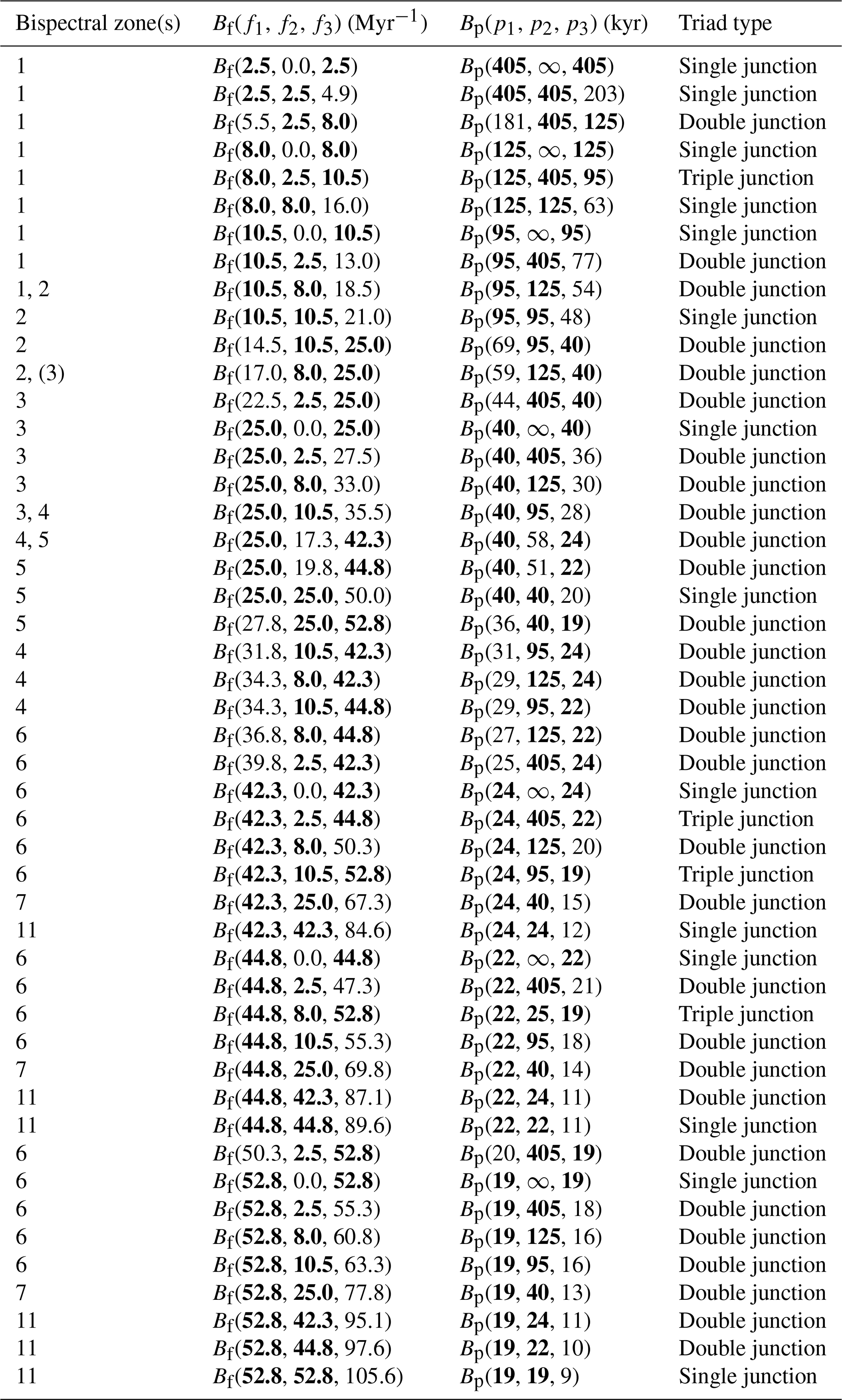
Table A2Bispectral triads among climate cycles with astronomical frequencies. One, two, or three astronomical frequencies (bold font) can partake in triad interactions, and we refer to these coordinates in the bispectrum as single, double, or triple junctions, respectively. These triads reflect positions in the frequency–frequency domain where nonlinear energy transfers among astronomically paced climate cycles are likely to occur. They correspond to the crossing points of the coloured lines in Fig. 3. In the case of a “single junction”, an astronomically paced cycle exchanges energy with itself or with a frequency that is only slightly offset. Single junctions where f1=f2 constitute the first higher harmonic interactions. Double or triple junctions are “combination tones” of two or three different astronomically paced cycles (Pestiaux et al., 1988; Hagelberg et al., 1991; King, 1996; Rial and Anaclerio, 2000).
The supplement related to this article is available online at: https://doi.org/10.5194/cp-15-1959-2019-supplement.
DL and ATMdB designed the study, made the figures and wrote the manuscript. ATMdB adjusted the MATLAB scripts for the purposes of this study.
The authors declare that they have no conflict of interest.
We thank Xavier Bertin for inviting Diederik Liebrand to present this work at an early stage at the Université de La Rochelle. We are grateful to Tim E. van Peer for making us aware of the difficulties in quantifying robust geometries of non-ergodic records. We thank Lorraine E. Lisiecki and Maureen E. Raymo, and Seonmin Ahn and colleagues for making their benthic foraminiferal δ18O stacks available online. We thank Thomas H. C. Herbers and Gerben Ruessink for providing bispectral analysis MATLAB scripts, which Anouk T. M. de Bakker developed further for the purposes of this study. We thank Qiuzhen Yin for the editorial handling of the manuscript. We thank Mathieu Martinez and the anonymous referee for their valuable comments during the review process.
The article processing charges for this open-access publication were covered by the University of Bremen.
This paper was edited by Qiuzhen Yin and reviewed by Mathieu Martinez and one anonymous referee.
Abe-Ouchi, A., Saito, F., Kawamura, K., Raymo, M. E., Okuno, J., Takahashi, K., and Blatter, H.: Insolation-driven 100 000-year glacial cycles and hysteresis of ice-sheet volume, Nature, 500, 190–194, https://doi.org/10.1038/nature12374, 2013.
Agassiz, L.: Études sur les glaciers, Neuchâtel, Jent et Gassmann, available at: https://archive.org/details/etudessurlesgla00agasgoog/page/n10 (last access: 30 March 2019), 1840.
Ahn, S., Khider, D., Lisiecki, L. E., and Lawrence, C. E.: A probabilistic Pliocene–Pleistocene stack of benthic δ18O using a profile hidden Markov model, Dynamics and Statistics of the Climate System, 2, 1–16, https://doi.org/10.1093/climsys/dzx002, 2017.
Bak, P.: How nature works: the science of self-organized criticality, Copernicus, New York, 1996.
Bak, P., Tang, C., and Wiesenfeld, K.: Self-organized criticality – an explanation of 1/f noise, Phys. Rev. Lett., 59, 381–384, https://doi.org/10.1103/PhysRevLett.59.381, 1987.
Bak, P., Tang, C., and Wiesenfeld, K.: Self-organized criticality, Phys. Rev. A, 38, 364–374, https://doi.org/10.1103/PhysRevA.38.364, 1988.
Beerling, D. J. and Royer, D. L.: Convergent Cenozoic CO2 history, Nat. Geosci., 4, 418–420, https://doi.org/10.1038/ngeo1186, 2011.
Berger, A., Loutre, M. F., and Mélice, J. L.: Equatorial insolation: from precession harmonics to eccentricity frequencies, Clim. Past, 2, 131–136, https://doi.org/10.5194/cp-2-131-2006, 2006.
Berger, A. L.: Support for astronomical theory of climatic change, Nature, 269, 44–45, https://doi.org/10.1038/269044a0, 1977.
Bintanja, R. and van de Wal, R. S. W.: North American ice-sheet dynamics and the onset of 100 000-year glacial cycles, Nature, 454, 869–872, https://doi.org/10.1038/nature07158, 2008.
Bosmans, J. H. C., Drijfhout, S. S., Tuenter, E., Hilgen, F. J., and Lourens, L. J.: Response of the North African summer monsoon to precession and obliquity forcings in the EC-Earth GCM, Clim. Dynam., 44, 279–297, https://doi.org/10.1007/s00382-014-2260-z, 2015a.
Bosmans, J. H. C., Hilgen, F. J., Tuenter, E., and Lourens, L. J.: Obliquity forcing of low-latitude climate, Clim. Past, 11, 1335–1346, https://doi.org/10.5194/cp-11-1335-2015, 2015b.
Broecker, W. S.: Absolute dating and astronomical theory of glaciation, Science, 151, 299–304, https://doi.org/10.1126/science.151.3708.299, 1966.
Calov, R. and Ganopolski, A.: Multistability and hysteresis in the climate-cryosphere system under orbital forcing, Geophys. Res. Lett., 32, L21717, https://doi.org/10.1029/2005GL024518, 2005.
Chalk, T. B., Hain, M. P., Foster, G. L., Rohling, E. J., Sexton, P. F., Badger, M. P. S., Cherry, S. G., Hasenfratz, A. P., Haug, G. H., Jaccard, S. L., Martinez-Garcia, A., Palike, H., Pancost, R. D., and Wilson, P. A.: Causes of ice age intensification across the Mid-Pleistocene Transition, P. Natl. Acad. Sci. USA, 114, 13114–13119, https://doi.org/10.1073/pnas.1702143114, 2017.
Chaudhuri, P. and Marron, J. S.: SiZer for exploration of structures in curves, J. Am. Stat. Assoc., 94, 807–823, https://doi.org/10.2307/2669996, 1999.
Cheng, H., Edwards, R. L., Sinha, A., Spotl, C., Yi, L., Chen, S. T., Kelly, M., Kathayat, G., Wang, X. F., Li, X. L., Kong, X. G., Wang, Y. J., Ning, Y. F., and Zhang, H. W.: The Asian monsoon over the past 640 000 years and ice age terminations, Nature, 534, 640–646, https://doi.org/10.1038/nature18591, 2016.
Clark, P. U. and Pollard, D.: Origin of the middle Pleistocene transition by ice sheet erosion of regolith, Paleoceanography, 13, 1–9, https://doi.org/10.1029/97pa02660, 1998.
Clark, P. U., Archer, D., Pollard, D., Blum, J. D., Rial, J. A., Brovkin, V., Mix, A. C., Pisias, N. G., and Roy, M.: The middle Pleistocene transition: characteristics. mechanisms, and implications for long-term changes in atmospheric pCO2, Quaternary Sci. Rev., 25, 3150–3184, https://doi.org/10.1016/j.quascirev.2006.07.008, 2006.
Collis, W. B., White, P. R., and Hammond, J. K.: Higher-order spectra: The bispectrum and trispectrum, Mech. Syst. Signal Pr., 12, 375–394, https://doi.org/10.1006/mssp.1997.0145, 1998.
Crowhurst, S. J., Palike, H., and Rickaby, R. E. M.: Carbonate ions, orbits and Mg/Ca at ODP 1123, Geochim. Cosmochim. Ac., 236, 384–398, https://doi.org/10.1016/j.gca.2018.03.013, 2018.
Crucifix, M.: Oscillators and relaxation phenomena in Pleistocene climate theory, Philos. T. R. Soc. A, 370, 1140–1165, https://doi.org/10.1098/rsta.2011.0315, 2012.
Da Silva, A. C., Dekkers, M. J., De Vleeschouwer, D., Hladil, J., Chadimova, L., Slavik, L., and Hilgen, F. J.: Millennial-scale climate changes manifest Milankovitch combination tones and Hallstatt solar cycles in the Devonian greenhouse world, Geology, 47, 19–22, https://doi.org/10.1130/G45511.1, 2018.
de Bakker, A. T. M., Tissier, M. F. S., and Ruessink, B. G.: Shoreline dissipation of infragravity waves, Cont. Shelf Res., 72, 73–82, https://doi.org/10.1016/j.csr.2013.11.013, 2014.
de Bakker, A. T. M., Herbers, T. H. C., Smit, P. B., Tissier, M. F. S., and Ruessink, B. G.: Nonlinear infragravity-wave interactions on a gently sloping laboratory beach, J. Phys. Oceanogr., 45, 589–605, https://doi.org/10.1175/JPO-D-14-0186.1, 2015.
de Bakker, A. T. M., Tissier, M. F. S., and Ruessink, B. G.: Beach steepness effects on nonlinear infragravity-wave interactions: A numerical study, J. Geophys. Res.-Oceans, 121, 554–570, https://doi.org/10.1002/2015jc011268, 2016.
de Boer, B., van de Wal, R. S. W., Lourens, L. J., and Bintanja, R.: Transient nature of the Earth's climate and the implications for the interpretation of benthic δ18O records, Palaeogeogr. Palaeocl., 335, 4–11, https://doi.org/10.1016/j.palaeo.2011.02.001, 2012.
deMenocal, P. B.: Plio-Pleistocene African climate, Science, 270, 53–59, https://doi.org/10.1126/science.270.5233.53, 1995.
Doering, J. C. and Bowen, A. J.: Parametrization of orbital velocity asymmetries of shoaling and breaking waves using bispectral analysis, Coast. Eng., 26, 15–33, https://doi.org/10.1016/0378-3839(95)00007-X, 1995.
Elderfield, H., Ferretti, P., Greaves, M., Crowhurst, S., McCave, I. N., Hodell, D. A., and Piotrowski, A. M.: Evolution of ocean temperature and ice volume through the mid-Pleistocene climate transition, Science, 337, 704–709, https://doi.org/10.1126/science.1221294, 2012.
Elgar, S. and Guza, R. T.: Observations of bispectra of shoaling surface gravity-waves, J. Fluid Mech., 161, 425–448, https://doi.org/10.1017/S0022112085003007, 1985.
Elgar, S.: Relationships involving third moments and bispectra of a harmonic process, IEEE T. Acoust. Speech, ASSP-35, 1725–1726, https://doi.org/10.1109/TASSP.1987.1165090, 1987.
Elgar, S. and Sebert, G.: Statistics of bicoherence and biphase, J. Geophys. Res.-Oceans, 94, 10993–10998, https://doi.org/10.1029/JC094iC08p10993, 1989.
Farmer, J. R., Honisch, B., Haynes, L. L., Kroon, D., Jung, S., Ford, H. L., Raymo, M. E., Jaume-Segui, M., Bell, D. B., Goldstein, S. L., Pena, L. D., Yehudai, M., and Kim, J.: Deep Atlantic Ocean carbon storage and the rise of 100 000-year glacial cycles, Nat. Geosci., 12, 355–360, https://doi.org/10.1038/s41561-019-0334-6, 2019.
Ganopolski, A. and Calov, R.: The role of orbital forcing, carbon dioxide and regolith in 100 kyr glacial cycles, Clim. Past, 7, 1415–1425, https://doi.org/10.5194/cp-7-1415-2011, 2011.
Ganopolski, A., Winkelmann, R., and Schellnhuber, H. J.: Critical insolation-CO2 relation for diagnosing past and future glacial inception, Nature, 529, 200–203, https://doi.org/10.1038/nature16494, 2016.
Hagelberg, T., Pisias, N., and Elgar, S.: Linear and nonlinear couplings between orbital forcing and the marine δ18O record during the late Neogene, Paleoceanography, 6, 729–746, https://doi.org/10.1029/91PA02281, 1991.
Hagelberg, T. K., Bond, G., and deMenocal, P.: Milankovitch band forcing of sub-milankovitch climate variability during the Pleistocene, Paleoceanography, 9, 545–558, https://doi.org/10.1029/94pa00443, 1994.
Hasselmann, K.: Stochastic climate models. Part I. Theory, Tellus, 28, 473–485, https://doi.org/10.3402/tellusa.v28i6.11316, 1976.
Hasselmann, K., Munk, W., and MacDonald, G.: Bispectra of ocean waves, in: Proceedings of the Symposium on Time Series Analysis, edited by: Rosenblatt, M., John Wiley, 125–139, 1963.
Haug, G. H. and Tiedemann, R.: Effect of the formation of the Isthmus of Panama on Atlantic Ocean thermohaline circulation, Nature, 393, 673–676, https://doi.org/10.1038/31447, 1998.
Hays, J. D., Imbrie, J., and Shackleton, N. J.: Variations in the Earth's orbit – Pacemaker of the ice ages, Science, 194, 1121–1132, https://doi.org/10.1126/science.194.4270.1121, 1976.
Herbers, T. H. C. and Burton, M. C.: Nonlinear shoaling of directionally spread waves on a beach, J. Geophys. Res.-Oceans, 102, 21101–21114, https://doi.org/10.1029/97jc01581, 1997.
Herbers, T. H. C., Russnogle, N. R., and Elgar, S.: Spectral energy balance of breaking waves within the surf zone, J. Phys. Oceanogr., 30, 2723–2737, https://doi.org/10.1175/1520-0485(2000)030<2723:SEBOBW>2.0.CO;2, 2000.
Hilgen, F. J., Lourens, L. J., Van Dam, J. A., Beu, A. G., Boyes, A. F., Cooper, R. A., Krijgsman, W., Ogg, J. G., Piller, W. E., and Wilson, D. S.: The Neogene Period, in: Geologic Time Scale 2012, vols. 1 and 2, edited by: Gradstein, F. M., Ogg, J. G., Schmitz, M. D., and Ogg, G. M., Elsevier, 923–978, 2012.
Huybers, P.: Glacial variability over the last two million years: an extended depth-derived agemodel, continuous obliquity pacing, and the Pleistocene progression, Quaternary Sci. Rev., 26, 37–55, https://doi.org/10.1016/j.quascirev.2006.07.013, 2007.
Huybers, P.: Combined obliquity and precession pacing of late Pleistocene deglaciations, Nature, 480, 229–232, https://doi.org/10.1038/nature10626, 2011.
Huybers, P. and Curry, W.: Links between annual, Milankovitch and continuum temperature variability, Nature, 441, 329–332, https://doi.org/10.1038/nature04745, 2006.
Huybers, P. and Tziperman, E.: Integrated summer insolation forcing and 40 000-year glacial cycles: The perspective from an ice-sheet/energy-balance model, Paleoceanography, 23, PA1208, https://doi.org/10.1029/2007pa001463, 2008.
Huybers, P. and Wunsch, C.: A depth-derived Pleistocene age model: Uncertainty estimates, sedimentation variability, and nonlinear climate change, Paleoceanography, 19, PA1028, https://doi.org/10.1029/2002pa000857, 2004.
Huybers, P. and Wunsch, C.: Obliquity pacing of the late Pleistocene glacial terminations, Nature, 434, 491–494, https://doi.org/10.1038/nature03401, 2005.
Kender, S., Ravelo, A. C., Worne, S., Swann, G. E. A., Leng, M. J., Asahi, H., Becker, J., Detlef, H., Aiello, I. W., Andreasen, D., and Hall, I. R.: Closure of the Bering Strait caused Mid-Pleistocene Transition cooling, Nat. Commun., 9, 5386, https://doi.org/10.1038/s41467-018-07828-0, 2018.
Kennedy, A. B., Chen, Q., Kirby, J. T., and Dalrymple, R. A.: Boussinesq modeling of wave transformation, breaking, and runup. I: 1D, J. Waterw. Port C., 126, 39–47, https://doi.org/10.1061/(ASCE)0733-950X(2000)126:1(39), 2000.
King, T.: Quantifying nonlinearity and geometry in time series of climate, Quaternary Sci. Rev., 15, 247–266, https://doi.org/10.1016/0277-3791(95)00060-7, 1996.
King Hagelberg, T. and Cole, J.: Determining the role of linear and nonlinear interactions in records of climate change: possible solar influences in annual to century-scale record, in: Proceedings of the eleventh annual Pacific climate (PACLIM) workshop, edited by: Isaacs, C. M., and Tharp, V. L., Interagency ecological program, California department of water resources, 47–54, 1995.
Konijnendijk, T. Y. M., Ziegler, M., and Lourens, L. J.: On the timing and forcing mechanisms of late Pleistocene glacial terminations: Insights from a new high-resolution benthic stable oxygen isotope record of the eastern Mediterranean, Quaternary Sci. Rev., 129, 308–320, https://doi.org/10.1016/j.quascirev.2015.10.005, 2015.
Köppen, W. and Wegener, A.: Die klimate der geologischen vorzeit., Gebrüder Borntraeger, Berlin, 1924.
Laskar, J., Robutel, P., Joutel, F., Gastineau, M., Correia, A. C. M., and Levrard, B.: A long-term numerical solution for the insolation quantities of the Earth, Astron. Astrophys., 428, 261–285, https://doi.org/10.1051/0004-6361:20041335, 2004.
Laskar, J., Fienga, A., Gastineau, M., and Manche, H.: La2010: A new orbital solution for the long term motion of the Earth, Astron. Astrophys., 532, A89, https://doi.org/10.1051/0004-6361/201116836, 2011a.
Laskar, J., Gastineau, M., Delisle, J.-B., Farrés, A., and Fienga, A.: Strong chaos induced by close encounters with Ceres and Vesta, Astron. Astrophys., 532, 1–4, https://doi.org/10.1051/0004-6361/201117504, 2011b.
Liebrand, D., de Bakker, A. T. M., Beddow, H. M., Wilson, P. A., Bohaty, S. M., Ruessink, G., Pälike, H., Batenburg, S. J., Hilgen, F. J., Hodell, D. A., Huck, C. E., Kroon, D., Raffi, I., Saes, M. J. M., van Dijk, A. E., and Lourens, L. J.: Evolution of the early Antarctic ice ages, P. Natl. Acad. Sci. USA, 114, 3867–3872, https://doi.org/10.1073/pnas.1615440114, 2017.
Lisiecki, L. E.: Links between eccentricity forcing and the 100 000-year glacial cycle, Nat. Geosci., 3, 349–352, https://doi.org/10.1038/Ngeo828, 2010.
Lisiecki, L. E. and Raymo, M. E.: A Pliocene-Pleistocene stack of 57 globally distributed benthic δ18O records, Paleoceanography, 20, PA1003, https://doi.org/10.1029/2004PA001071, 2005a.
Lisiecki, L. E. and Raymo, M. E.: Pliocene-Pleistocene stack of globally distributed benthic stable oxygen isotope records, PANGAEA, https://doi.org/10.1594/PANGAEA.704257, 2005b.
Lisiecki, L. E. and Raymo, M. E.: Plio-Pleistocene climate evolution: trends and transitions in glacial cycle dynamics, Quaternary Sci. Rev., 26, 56–69, https://doi.org/10.1016/j.quascirev.2006.09.005, 2007.
Lisiecki, L. E., Raymo, M. E., and Curry, W. B.: Atlantic overturning responses to Late Pleistocene climate forcings, Nature, 456, 85–88, https://doi.org/10.1038/nature07425, 2008.
Liu, Z., Otto-Bliesner, B. L., He, F., Brady, E. C., Tomas, R., Clark, P. U., Carlson, A. E., Lynch-Stieglitz, J., Curry, W., Brook, E., Erickson, D., Jacob, R., Kutzbach, J., and Cheng, J.: Transient Simulation of Last Deglaciation with a New Mechanism for Bolling-Allerod Warming, Science, 325, 310–314, https://doi.org/10.1126/science.1171041, 2009.
Lourens, L. J. and Hilgen, F. J.: Long-periodic variations in the Earth's obliquity and their relation to third-order eustatic cycles and late Neogene glaciations, Quatern. Int., 40, 43–52, https://doi.org/10.1016/S1040-6182(96)00060-2, 1997.
Lourens, L. J., Becker, J., Bintanja, R., Hilgen, F. J., Tuenter, E., van de Wal, R. S. W., and Ziegler, M.: Linear and non-linear response of late Neogene glacial cycles to obliquity forcing and implications for the Milankovitch theory, Quaternary Sci. Rev., 29, 352–365, https://doi.org/10.1016/j.quascirev.2009.10.018, 2010.
Martinez-Boti, M. A., Foster, G. L., Chalk, T. B., Rohling, E. J., Sexton, P. F., Lunt, D. J., Pancost, R. D., Badger, M. P. S., and Schmidt, D. N.: Plio-Pleistocene climate sensitivity evaluated using high-resolution CO2 records, Nature, 518, 49–54, https://doi.org/10.1038/nature14145, 2015.
Meyers, S. R. and Hinnov, L. A.: Northern Hemisphere glaciation and the evolution of Plio-Pleistocene climate noise, Paleoceanography, 25, PA3207, https://doi.org/10.1029/2009pa001834, 2010.
Milankovitch, M.: Canon of Insolation and the Ice-Age Problem, 1st ed., Zavod za udžbenike i nastavna sredstva & Muzej nauke i tehnike Srpske akademije nauka i umetnosti, Beograd, 1941.
Muller, R. A. and MacDonald, G. J.: Spectrum of 100 kyr glacial cycle: Orbital inclination, not eccentricity, P. Natl. Acad. Sci. USA, 94, 8329–8334, https://doi.org/10.1073/pnas.94.16.8329, 1997a.
Muller, R. A. and MacDonald, G. J.: Simultaneous presence of orbital inclination and eccentricity in proxy climate records from Ocean Drilling Program Site 806, Geology, 25, 3–6, https://doi.org/10.1130/0091-7613(1997)025<0003:SPOOIA>2.3.CO;2, 1997b.
Norheim, C. A., Herbers, T. H. C., and Elgar, S.: Nonlinear evolution of surface wave spectra on a beach, J. Phys. Oceanogr., 28, 1534–1551, https://doi.org/10.1175/1520-0485(1998)028<1534:Neosws>2.0.Co;2, 1998.
Paillard, D., Labeyrie, L., and Yiou, P.: AnalySeries, Macintosh program performs time-series analysis, EOS Transactions AGU, 77, 379, https://doi.org/10.1029/96EO00259, 1996.
Pelletier, J. D.: The power spectral density of atmospheric temperature from time scales of 10−2 to 106 yr, Earth Planet. Sc. Lett., 158, 157–164, https://doi.org/10.1016/S0012-821x(98)00051-X, 1998.
Pestiaux, P., Van der Mersch, I., Berger, A., and Duplessy, J. C.: Paleoclimatic variability at frequencies ranging from 1 cycle per 10 000 years to 1 cycle per 1000 years: evidence for nonlinear behaviour of the climate system, Climatic Change, 12, 9–37, https://doi.org/10.1007/Bf00140262, 1988.
Pisias, N. G., Mix, A. C., and Zahn, R.: Nonlinear response in the global climate system: evidence from benthic oxygen isotopic record in Core Rc13-110, Paleoceanography, 5, 147–160, https://doi.org/10.1029/PA005i002p00147, 1990.
Raymo, M. E. and Nisancioglu, K.: The 41 kyr world: Milankovitch's other unsolved mystery, Paleoceanography, 18, 1011, https://doi.org/10.1029/2002pa000791, 2003.
Raymo, M. E., Lisiecki, L. E., and Nisancioglu, K. H.: Plio-pleistocene ice volume, Antarctic climate, and the global δ18O record, Science, 313, 492–495, https://doi.org/10.1126/science.1123296, 2006.
Rial, J. A. and Anaclerio, C. A.: Understanding nonlinear responses of the climate system to orbital forcing, Quaternary Sci. Rev., 19, 1709–1722, https://doi.org/10.1016/S0277-3791(00)00087-1, 2000.
Ridgwell, A. J., Watson, A. J., and Raymo, M. E.: Is the spectral signature of the 100 kyr glacial cycle consistent with a Milankovitch origin?, Paleoceanography, 14, 437–440, https://doi.org/10.1029/1999pa900018, 1999.
Roe, G.: In defense of Milankovitch, Geophys. Res. Lett., 33, L24703, https://doi.org/10.1029/2006gl027817, 2006.
Roe, G. H. and Allen, M. R.: A comparison of competing explanations for the 100 000-yr ice age cycle, Geophys. Res. Lett., 26, 2259–2262, https://doi.org/10.1029/1999gl900509, 1999.
Rohling, E. J., Foster, G. L., Grant, K. M., Marino, G., Roberts, A. P., Tamisiea, M. E., and Williams, F.: Sea-level and deep-sea-temperature variability over the past 5.3 million years, Nature, 508, 477–482, https://doi.org/10.1038/nature13230, 2014.
Rutherford, S. and D'Hondt, S.: Early onset and tropical forcing of 100 000-year Pleistocene glacial cycles, Nature, 408, 72–75, https://doi.org/10.1038/35040533, 2000.
Shackleton, N. J.: The 100 000-year ice-age cycle identified and found to lag temperature, carbon dioxide, and orbital eccentricity, Science, 289, 1897–1902, https://doi.org/10.1126/science.289.5486.1897, 2000.
Sun, Y., Chen, J., Clemens, S. C., Liu, Q. S., Ji, J. F., and Tada, R.: East Asian monsoon variability over the last seven glacial cycles recorded by a loess sequence from the northwestern Chinese Loess Plateau, Geochem. Geophy. Geosy., 7, Q12Q02, https://doi.org/10.1029/2006gc001287, 2006.
Tabor, C. R. and Poulsen, C. J.: Simulating the mid-Pleistocene transition through regolith removal, Earth Planet. Sc. Lett., 434, 231–240, https://doi.org/10.1016/j.epsl.2015.11.034, 2016.
Tziperman, E., Raymo, M. E., Huybers, P., and Wunsch, C.: Consequences of pacing the Pleistocene 100 kyr ice ages by nonlinear phase locking to Milankovitch forcing, Paleoceanography, 21, PA4206, https://doi.org/10.1029/2005pa001241, 2006.
Viaggi, P.: δ18O and SST signal decomposition and dynamic of the Pliocene-Pleistocene climate system: new insights on orbital nonlinear behavior vs. long-term trend, Progress in Earth and Planetary Science, 5, 1–37, https://doi.org/10.1186/s40645-018-0236-z, 2018.
von Dobeneck, T. and Schmieder, F.: Using rock magnetic proxy records for orbital tuning and extended time series analyses into the super- and sub-Milankovitch band, in: Use of proxies in paleoceanography: examples from the South Atlantic, edited by: Fischer, G. and Wefer, G., Springer-Verlag, Berlin, Heidelberg, 601–633, https://doi.org/10.1007/978-3-642-58646-0_25, 1999.
Wara, M. W., Ravelo, A. C., and Revenaugh, J. S.: The pacemaker always rings twice, Paleoceanography, 15, 616–624, https://doi.org/10.1029/2000pa000500, 2000.
Werner, M., Heimann, M., and Hoffmann, G.: Isotopic composition and origin of polar precipitation in present and glacial climate simulations, Tellus B, 53, 53–71, https://doi.org/10.3402/tellusb.v53i1.16539, 2001.
Willeit, M., Ganopolski, A., Calov, R., Robinson, A., and Maslin, M.: The role of CO2 decline for the onset of Northern Hemisphere glaciation, Quaternary Sci. Rev., 119, 22–34, https://doi.org/10.1016/j.quascirev.2015.04.015, 2015.
Willeit, M., Ganopolski, A., Calov, R., and Brovkin, V.: Mid-Pleistocene transition in glacial cycles explained by declining CO2 and regolith removal, Sci. Adv., 5, eaav7337, https://doi.org/10.1126/sciadv.aav7337, 2019.
Wu, P. L., Jackson, L., Pardaens, A., and Schaller, N.: Extended warming of the northern high latitudes due to an overshoot of the Atlantic meridional overturning circulation, Geophys. Res. Lett., 38, L24704, https://doi.org/10.1029/2011gl049998, 2011.
Yiou, P., Ghil, M., Jouzel, J., Paillard, D., and Vautard, R.: Nonlinear variability of the climatic system from singular and power spectra of late Quaternary records, Clim. Dynam., 9, 371–389, https://doi.org/10.1007/s003820050030, 1994.
Ziegler, M., Lourens, L. J., Tuenter, E., Hilgen, F., Reichart, G. J., and Weber, N.: Precession phasing offset between Indian summer monsoon and Arabian Sea productivity linked to changes in Atlantic overturning circulation, Paleoceanography, 25, PA3213, https://doi.org/10.1029/2009pa001884, 2010.