the Creative Commons Attribution 4.0 License.
the Creative Commons Attribution 4.0 License.
 | 18 Feb 2019
Harmonising plant functional type distributions for evaluating Earth system models
Anne Dallmeyer
Martin Claussen
Victor Brovkin
Dynamic vegetation models simulate global vegetation in terms of fractional coverage of a few plant functional types (PFTs). Although these models often share the same concept, they differ with respect to the number and kind of PFTs, complicating the comparability of simulated vegetation distributions. Pollen-based vegetation reconstructions are initially only available in the form of time series of individual taxa that are not distinguished in the models. Thus, to evaluate simulated vegetation distributions, the modelling results and pollen-based vegetation reconstructions have to be converted into a comparable format. The classical approach is the method of biomisation, but hitherto PFT-based biomisation methods were only available for individual models. We introduce and evaluate a simple, universally applicable technique to harmonise PFT distributions by assigning them into nine mega-biomes, using only assumptions on the minimum PFT cover fractions and few bioclimatic constraints (based on the 2 m temperature). These constraints mainly follow the limitation rules used in the classical biome models (here BIOME4). We test the method for six state-of-the-art dynamic vegetation models that are included in Earth system models based on pre-industrial, mid-Holocene and Last Glacial Maximum simulations. The method works well, independent of the spatial resolution or the complexity of the models. Large biome belts (such as tropical forest) are generally better represented than regionally confined biomes (warm–temperate forest, savanna). The comparison with biome distributions inferred via the classical biomisation approach of forcing biome models (here BIOME1) with the simulated climate states shows that the PFT-based biomisation is even able to keep up with the classical method. However, as the new method considers the PFT distributions actually calculated by the Earth system models, it allows for a direct comparison and evaluation of simulated vegetation distributions which the classical method cannot do. Thereby, the new method provides a powerful tool for the evaluation of Earth system models in general.


Within dynamic global vegetation models (DGVMs), the natural vegetation distribution is usually represented in the form of plant functional types (PFTs); i.e. plants are grouped with regard to their physiology and physiognomy (Prentice et al., 2007). These PFTs differ with respect to phenology, albedo, morphological and photosynthetic parameters and are usually constrained by an individual bioclimatic range of tolerance defined by temperature thresholds. These thresholds represent the cold resistance, chilling and heat requirements of the plants and determine the area where the PFTs can be established.
In most DGVMs, a “mosaic” approach is used; i.e. each grid box of the land surface is split into separate parts for a non-vegetated and a vegetated fraction that is further tiled in mosaics, taking subgrid-scale heterogeneity into account. Thus, several PFTs can cover the same grid cell and compete for space via their net primary productivity (e.g. Sitch et al., 2003; Krinner et al., 2005; Reick et al., 2013). Non-vegetated area (seasonally bare soil or permanently bare ground) is produced where plant productivity is too low.
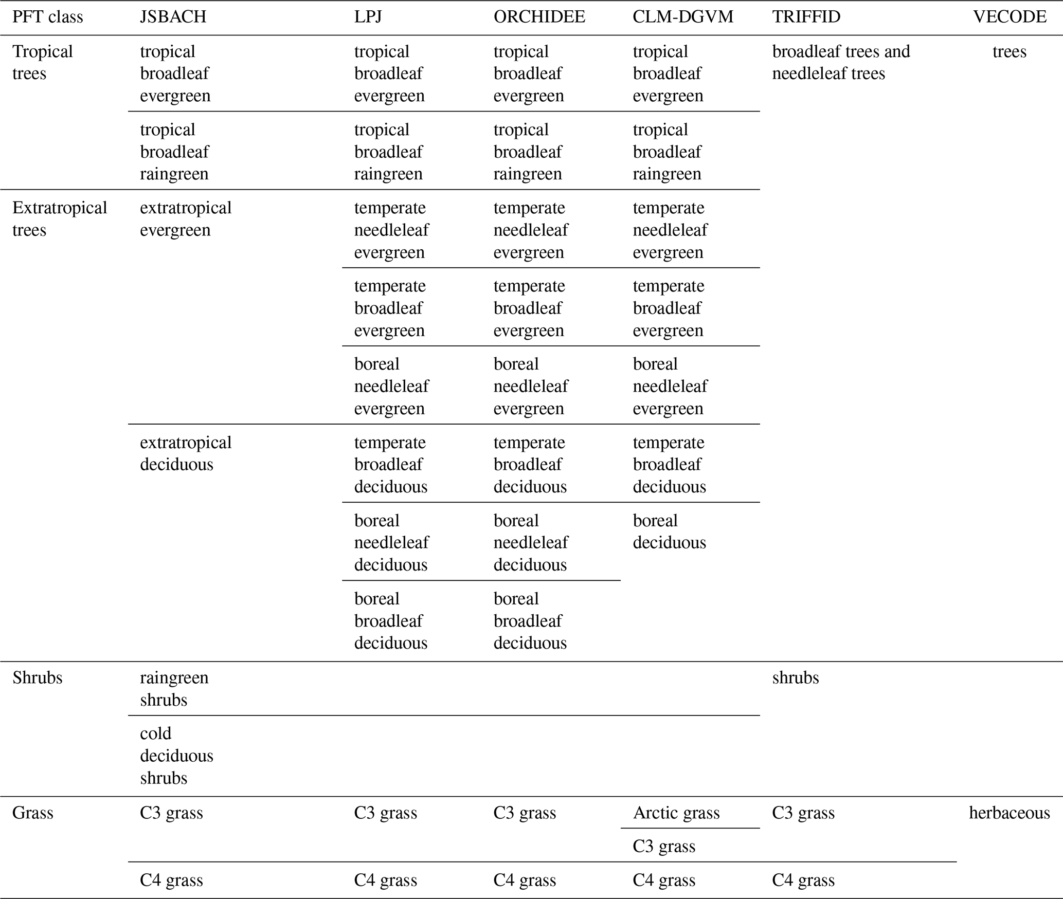
Although the main principles for the calculation of PFT distributions are similar among most DGVMs, they vary regarding the number and kind of PFTs used to represent the global vegetation. Natural (non-anthropogenic) PFTs range from 2 in, e.g. VECODE (for definition of the acronyms of the DGVMs, see Table 1), to 10 in, e.g. LPJ and ORCHIDEE (Table 1). Even within the same model, PFT variety can differ between individual simulations, e.g. due to the inclusion of land-use types. These differences among the simulations and models prohibit the intermodel comparability of simulated global vegetation distributions and the comparability with pollen-based biome reconstructions.
Table 1The PFTs used in the different state-of-the-art dynamic global vegetation models. These are the Jena Scheme for Biosphere Atmosphere Coupling in Hamburg (JSBACH), the Lund–Potsdam–Jena model (LPJ), the Organising Carbon and Hydrology In Dynamic Ecosystems model (ORCHIDEE), the Community Land Model's dynamic global vegetation model (CLM-DGVM), the Top-down Representation of Interactive Foliage and Flora Including Dynamics (TRIFFID) model and the Vegetation Continuous Description model (VECODE).
Pollen records are originally displayed in the form of pollen percentages or pollen accumulation rates, what cannot be directly compared to plant functional type distributions, as pollen records do not reflect the actual plant abundances. For a systematic comparison of simulated plant functional type distributions and reconstructions, both need to be converted in a compatible format. In the last two decades, taxa to PFT assignment methods and the method of “biomisation” for pollen-based reconstructions have been developed (e.g. Prentice et al., 1996; Ni et al., 2010; Harrison et al., 2010), so that pollen assemblages can be grouped into biomes (e.g. tropical forest, temperate steppe, desert). Pollen-based biome syntheses have been provided (Prentice et al., 1998, 2000; Bigelow et al., 2003; Ni et al., 2010; Harrison, 2017; Tian et al., 2017) that have extensively been used to evaluate simulated biome distributions obtained from diagnostic biome models such as BIOME1 or BIOME4 (e.g. Prentice et al., 1992; Haxeltine and Prentice, 1996; Kaplan et al., 2003). These biome models can be forced by observed or simulated climate fields and calculate biome distributions in equilibrium to this input climate. Using this classical method of biomisation, fundamental palaeo-vegetation analysis can be undertaken (e.g. Jolly et al., 1998; Harrison et al., 2003, 2016; Wohlfahrt et al., 2008; Dallmeyer et al., 2017) without requiring an explicit calculated vegetation distribution by the Earth system models (ESMs). On the other hand, this also means that existing simulated plant functional type distributions calculated by the DGVMs being dynamically coupled in these models are neglected, since only the simulated climate pattern is taken into account. The biomisation via diagnostic biome models did not include any information on the original PFT distribution simulated by the Earth system models. As the DGVMs are generally more complex than the biome models and include more relevant processes, valuable information included in the PFT distribution gets lost in the classical biomisation by the biome models. A more appropriate method of biomisation would be to directly use the PFT distributions calculated by the DGVMs.
Several model studies have taken up this problem by introducing methods for biomising PFT distributions simulated by DGVMs. Schurgers et al. (2006) derive biome maps for the Eemian and mid-Holocene from the relative fractional coverage of the individual PFTs and the soil temperature, both simulated by LPJ. With this method, reconstructed major biome shifts could be reproduced. Roche et al. (2007) used the dominant PFT and the bioclimate limits defined in the biome model BIOME1 (Prentice et al., 1992) to biomise PFT cover fractions for the Last Glacial Maximum (LGM) simulated by VECODE. As VECODE distinguishes as main PFTs only trees and herbaceous plants, not all biome types defined in BIOME1 could be considered (e.g. no shrubs). The computed biome map shows reasonable agreement with LGM land cover reconstructions. A similar approach was chosen by Handiani et al. (2012, 2013) for calculating biome distributions during Heinrich event 1, based on PFT simulations of TRIFFID and CLM-DGVM. As these models strongly deviate in their PFT classification, they applied different methods for biomisation. For TRIFFID, they first calculated the dominant PFT in each grid cell following the method by Crucifix et al. (2005) and afterwards used temperature limitation defined in BIOME4 (Kaplan et al., 2003) to assign the dominant PFTs to mega-biomes. For CLM-DGVM, potential dominant PFTs were estimated by adopting the scheme of Schurgers et al. (2006) and biomes were differentiated with the help of temperature limitations that follow the environmental constraints defined in CCSM3 (i.e. the fully coupled model used in their study, including the land and vegetation model CLM-DGVM).
Recently, Prentice et al. (2011) introduced another approach of biomising plant functional type distributions simulated by dynamic vegetation models. In their method, simulated foliage projective cover (FPC) is used to distinguish between desert, grassland/dry shrubland and forest biomes, which are further divided into forest and savanna-like biomes through the vegetation height. The assignment to, e.g. boreal, temperate or tropical forest/savanna (or parkland) is controlled by the tree-PFT composition. Climate limits are only used to distinguish the tundra biome. This method has successfully been used in several palaeo-vegetation studies (Kageyama et al., 2013; Calvo and Prentice, 2015) using different versions of the LPJ and ORCHIDEE models.
All of these methods have in common that they have been designed for individual models and hence need specific output not necessarily provided by all models. Therefore, these methods cannot directly be adopted for all existing dynamic vegetation models. A consistent intermodel comparison of the simulated vegetation distribution and an evaluation of the models against reconstructions on biome level is so far not possible.
To harmonise (palaeo)-vegetation distributions simulated by dynamic vegetation models and thereby facilitate the evaluation of Earth system models (ESMs) and the comparison of model results and biome reconstructions, we developed a biomisation technique that is based on the PFT distributions simulated by DGVMs, few input variables and simple differentiation rules. These include bioclimatic constraints using near-surface air temperature and assumptions on maximum required PFT coverage. The aim of developing this method was not to construct a better biomisation method than the classical method via diagnostic biome models but to develop a more direct method that can convert PFT distributions into biomes so that the additional information included due to the coupling of the DGVM will not get lost.
We test this method on pre-industrial, mid-Holocene and Last Glacial Maximum vegetation simulations performed in nearly all state-of-the-art dynamic vegetation models. The skill of this biomisation approach is quantified via (standard) metrics, by comparing the converted biome maps with estimates of modern potential biome distributions (Ramankutty and Foley, 1999) and pollen-based biome reconstructions (Biome6000 database, Harrison, 2017).
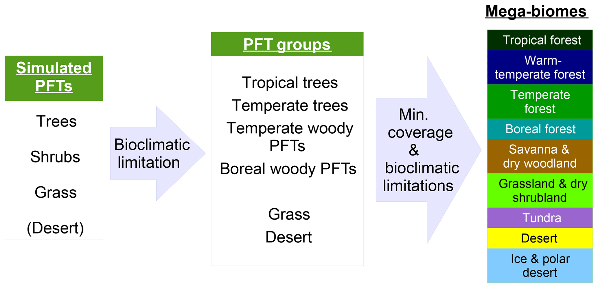
Figure 1Scheme of the biomisation method. The PFT fractions simulated by the individual DGVMs are assigned to the PFT groups “desert” (i.e. 1 minus total vegetation), “grass” (containing all grass PFT types) “woody PFT” (containing all trees and shrub types) and “trees” (containing all tree types). The “trees” and “woody PFTs” are further differentiated into “tropical trees”, “temperate trees”, “temperate woody PFTs” and “boreal woody PFTs” via bioclimatic limitations (Table 2). For DGVMs explicitly distinguishing tropical, temperate or boreal tree types, the original classification of the DGVM is used. Afterwards, the PFT groups are assigned to nine mega-biomes by assumptions on the minimum coverage of certain PFT groups needed in a grid cell and additional bioclimatic limitations (Table 2).
2.1 Biomisation
The PFT cover fractions simulated by the individual dynamic vegetation models are converted into nine different mega-biomes (Fig. 1), using few bioclimatic limits and assumptions on the maximum required coverage of certain PFTs. The aggregation into the mega-biomes is in line with the definitions of the BIOME6000 project (cf. Harrison, 2017) that are also commonly used for grouping pollen-based biome reconstructions. Bioclimatic limits and the differentiation rules basically follow the biome assignment of the BIOME4 model (Kaplan et al., 2003). As input data, only climatological mean growing degree days (GDD0 and GDD5), monthly mean 2 m air temperature and multi-year mean PFT cover fractions (e.g. averaged over 100 years) are required. The limitation to few climatic rules and few variables needed enables the application of the method to all state-of-the-art dynamic vegetation models.
In detail, the PFTs calculated by the respective dynamic vegetation models are aggregated into the groups “trees”, “woody PFTs” (i.e. shrubs and all tree PFTs), “grass” and “desert”, which is calculated as 1 minus the total vegetation. If the model includes land-use types, the affected areas are redistributed to the other PFTs by simply scaling up the other PFT fractions proportionally to their ratio of the total natural vegetation. Based on these groups, regions dominated by trees and regions in which the cover fraction of the woody PFTs exceeds 25 % (with the additional constraint of the total vegetation cover exceeding 50 %) are identified, as these are necessary conditions for the assignment of the land cover to forest biomes. Afterwards, the groups “trees” and “woody PFTs” are split into boreal (GDD5 ≤ 900 ∘C), temperate (GDD5 > 900 ∘C) and tropical trees or woody PFTs (Tc > 15.5 ∘C) via temperature limits (cf. Table 2). If any of these tree PFTs are simulated directly in the vegetation model (e.g. in LPJ or ORCHIDEE), the original distributions are taken and the PFT group is assigned to the dominant tree type, i.e. the tree type that covers the largest fraction of the grid cell. These PFT groups (i.e. boreal woody PFTs, temperate trees and woody PFTs, tropical trees, grass and desert) are the first consistent vegetation classification shared by all input simulations, so that model-to-model comparison is also possible on this PFT level.
Table 2Bioclimatic limits and assumptions on minimum PFT coverage needed for the assignment of PFTs into the PFT groups and into the nine mega-biomes. The separation of boreal, temperate and tropical tree PFTs is based on the same bioclimatic limits as the respective forest mega-biomes. Only temperature-based limitations are used, i.e. the growing degree days on a basis of 5 ∘C (GDD5) or on a basis of 0 ∘C (GDD0), the monthly mean temperature of the coldest month (Tc) and the annual mean temperature (Tann). Bioclimatic limits are mainly taken from the BIOME4 model (Kaplan et al., 2003, marked with *). The limit for tropical forest is taken from BIOME1 (Prentice et al., 1992) but is also commonly used in DGVMs (e.g. JSBACH). The limit for the differentiation of deserts has been empirically determined in this study and is close to the value chosen by Handiani et al. (2013) and within the range of the Köppen–Geiger climate classification for polar climate and the Holdridge alpine life zone classification. The Tc limit for warm savannas is taken from JSBACH (C4 grass criteria) to exclude temperate savannas. The assumptions on minimum coverage have been partly taken, partly empirically adapted from Handiani et al. (2013). A flow chart displaying the biomisation procedure is shown in Appendix A for the VECODE model, the DGVM used in the CLIMate-BiosphERe 2 (CLIMBER-2) model.
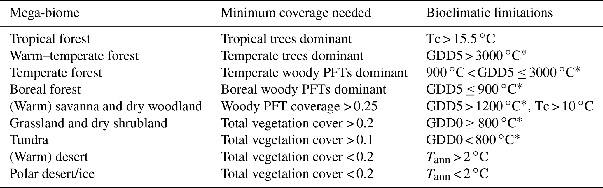
For the biomisation, the forests are considered first; i.e. regions in which trees or woody PFTs are dominant or cover an area more than 25 % are assigned to tropical, temperate and boreal forests according to the PFT groups. From the temperate forest, warm regions (i.e. GDD5 > 3000 ∘C) revealing a dominant temperate tree fraction are subtracted and assigned to the biome “warm–temperate forest”. The remaining area is then tested for fulfilling the constraints for the non-forest biomes. First, the savanna and dry woodland region is identified by bioclimatic limitations (GDD5 > 1200 and Tc > 10 ∘C) and a woody PFT coverage of at least 25 %. The remaining vegetated area is assigned to the biome “grassland and dry shrublands”, if GDD0 exceeds 800 ∘C, or to the biome “tundra”, if GDD0 is below 800 ∘C (cf. BIOME4; Kaplan et al., 2003). The non-vegetated area, i.e. regions in which the total vegetation cover is less than 20 %, is either assigned to warm or to cold desert, depending on whether the annual mean temperature is above or below 2 ∘C. For the biome “tundra”, only 10 % vegetation cover is needed. A flow chart summarising the details of the PFT-based biomisation is shown for the VECODE model in Appendix A.
We are aware of the simplicity of this approach, calculating the tundra and the grassland and dry shrubland biomes as a residual of the non-forested area, not directly depending on the simulated grass PFT fraction. We decided to attribute the main priority to the forested biomes as this is also the strategy commonly used in DGVMs and biome models.
To assess the performance of the biomisation based on simulated PFTs, we additionally biomise the simulated climate fields corresponding to the PFT distributions in each model. This is the conventionally used procedure to biomise general circulation model (GCM) or ESM output (further referred to as the classical approach or climate-based method). For this purpose, we use the biome model BIOME1 (Prentice et al., 1992) that calculates the biome distribution in equilibrium to the input climate. As forcing, BIOME1 needs the monthly mean climatological precipitation, near-surface temperature and cloudiness, which were taken from each simulation considered in this study, respectively. This classical biomisation approach can only handle climate data as input; the simulated PFT distributions from the ESMs used in the here-introduced PFT-based method are ignored. The original biomes have been grouped into the same mega-biome classification that is used for the PFT-based approach.
2.2 Simulations
Simulations from nearly all state-of-the-art global dynamic vegetation models that are included in Earth system models have been selected for biomisation. Six different models could be considered (i.e. JSBACH, TRIFFID, ORCHIDEE, SEIB, LPJ and VECODE). Overall, eight simulations for the pre-industrial climate (PI) and vegetation, four for mid-Holocene (6 ka) conditions and five for Last Glacial Maximum (LGM) conditions have been used (Table 3). Most of these simulations were performed within CMIP5/PMIP3 under strict simulation and output protocols enabling direct comparison between the models (Braconnot et al., 2011; Taylor et al., 2012). These include the models MPI-ESM-P, IPSL-CM5A-LR, MIROC-ESM and HadGem2-ESM. Further details on the models and simulations are described in Appendix B.
Table 3Overview of the simulations used for testing the biomisation method. Listed are the model acronym, the model name, the name of the included DGVM, the simulations used in this study, the spatial resolution used in the simulations, the number of PFTs (natural plus anthropogenic) and the simulation reference. Simulations marked with the * symbol include land use. Simulations marked with the # symbol ran with prescribed vegetation.
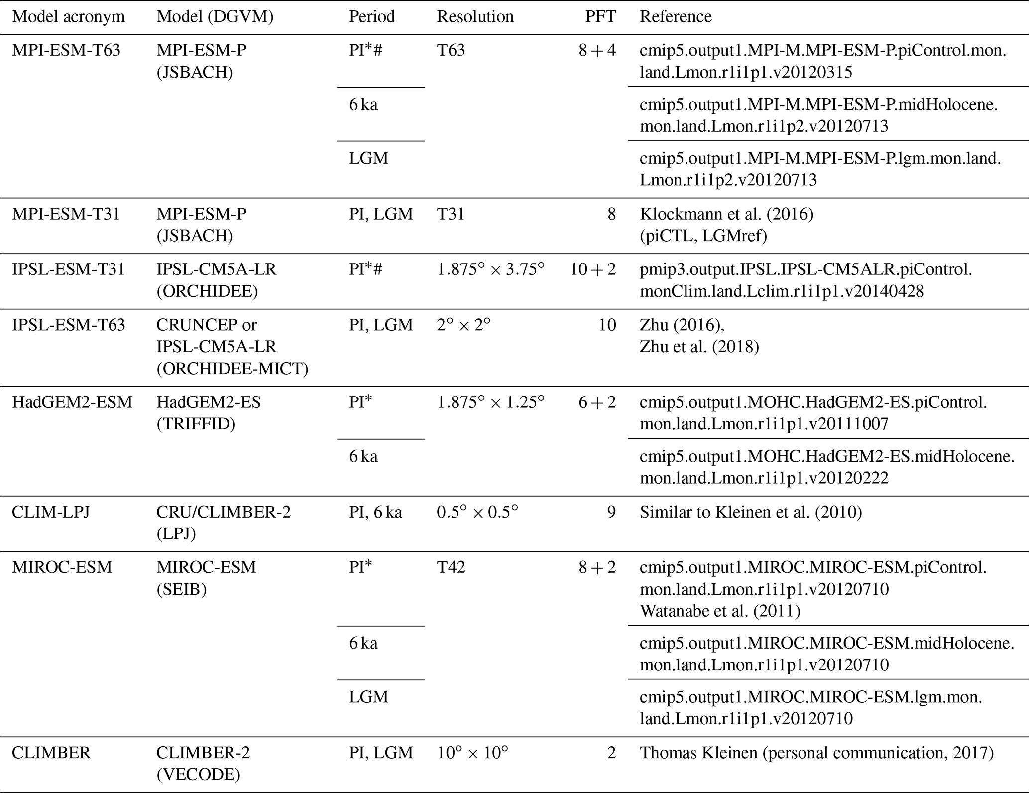
For the pre-industrial time slice, two out of eight simulations (MPI-ESM-T63 and IPSL-ESM-T31) were performed with fixed vegetation distribution, but this has essentially no effect on the biomisation procedure. Therefore, we include these simulations in our analysis. Nevertheless, the PFT-based biome distributions for these simulations are expected to fit better to the references than the other simulations that ran with interactive vegetation.
We emphasise that this study is thought of as an introduction and detailed evaluation of a new biomisation method. It is not seen as evaluation of the different vegetation models with respect to the skill of simulating biome or vegetation distributions. For this purpose, the different vegetation models would have to be forced by the same climate state. Such an ensemble including all DGVMs (used here) does not exist. Therefore, we had to take individual simulations that all deviate with respect to the prescribed or simulated climate in the coupled models. These differences in the climatic field among the models and between the models and observations (general climate biases) lead – per se – to differences in the simulated vegetation distributions and biases to the reference vegetation distribution.
2.3 Preparing the reference datasets
As reference, we use the estimated global potential natural vegetation map by Ramankutty and Foley (1999, referred to as RF99 in the following), which is a combination of modern satellite-based vegetation observations (i.e. the DISCover land cover dataset) and the vegetation compilation prepared by Haxeltine and Prentice (1996) that has been taken for regions dominated by land use at present day. The RF99 dataset is available at 5 min resolution and distinguishes 15 different biome types that are similar to the mega-biome classification used here. Thus, most biomes could directly be assigned to the mega-biome types (Table C1 in Appendix C). The preparation of the RF99 reference dataset is explained in more detail in Appendix C.
As further reference data, we use pollen-based biome reconstructions that are available for the modern, mid-Holocene and Last Glacial Maximum time slices within the Biome6000 database (Harrison, 2017). The biome reconstructions have been grouped into the mega-biomes according to the suggestions made by the Biome6000 project.
Both vegetation datasets are derived for the modern time slice not exactly corresponding to the pre-industrial period (around 1850 AD) simulated in the models. While the ice sheet, the topography and the orbital conditions used for the pre-industrial control simulations are prescribed from modern conditions, greenhouse gases are set to pre-industrial values in the models. These differences in, e.g. atmospheric CO2 concentration between the reference datasets and the simulations may lead to small discrepancies in the model. In addition, the references may be disturbed by anthropogenic influences.
Climatological monthly mean data of the years 1901–1930 from the University of East Anglia Climate Research Unit Time Series 4.00 (CRU TS4, University of East Anglia, 2017) have been taken as the pre-industrial reference climate. This is the earliest period available. The CRU TS4 reference climate has additionally been used as forcing for the BIOME1 model to provide a best guess for the pre-industrial biome map. We assume that neither the biomisation of simulated climate states (i.e. the classical method) nor the biomisation of simulated PFTs can agree better with any reference than this biome distribution, derived with a highly tuned biome model and the best global climate observation available. Therefore, we use the level of agreement between the CRU TS4 biome map and the RF99 or the Biome6000 reconstructions as target value for our new biomisation method. The reference biome distributions and the CRU TS4-based biome map are displayed in Fig. 2.
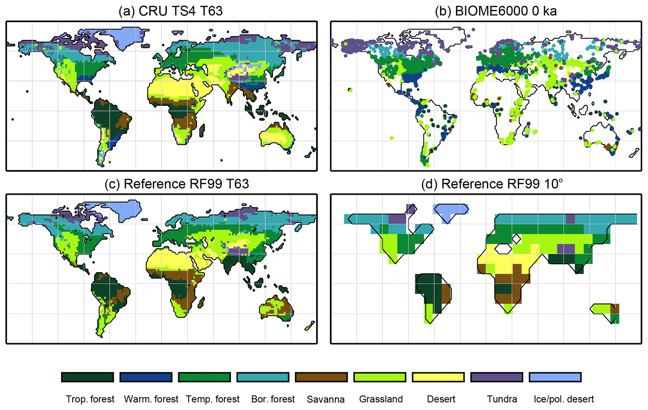
Figure 2Reference biome distributions for the pre-industrial time slice, i.e. (a) the biome distribution inferred by BIOME1 that has been forced by the CRU TS4 dataset (1901–1930), interpolated to a Gaussian T63 grid; (b) the pollen-based pre-industrial biome reconstructions provided by the Biome6000 database (Harrison, 2017); (c, d) the modern potential natural vegetation map derived by Ramankutty and Foley (1999, RF99) remapped on a T63 gaussian grid (c) and a 10∘ grid (d). The biomes are tropical forest (trop.forest), warm–temperate forest (warm.forest), temperate forest (temp.forest), boreal forest (bor.forest), savanna and dry woodland (savanna), grassland and dry shrubland (grassland), warm desert (desert), tundra (tundra) and polar desert and ice (ice/pol.desert).
2.4 Metrics
2.4.1 Kappa statistic
The kappa statistic (Cohen, 1960) is a widely used quantitative map-comparison technique that has often been applied for assessing the performance of vegetation simulations (e.g. Monserud and Leemans, 1992; Prentice et al., 1992; Diffenbaugh et al., 2003; Tang et al., 2009). The kappa statistic not only includes the actual observed similarity (p0) of two categorical maps but also considers the expected agreement (pe), i.e. the agreement by chance. For each pair of compared grid cells (or a pair of grid cell and site) taken from the reference and the simulated biome distributions, a confusion matrix is prepared containing all combinations of referenced and simulated biomes. Based on this error matrix, the agreement for each individual mega-biome is given by the following (Eq. 1, taken from Tang et al., 2009):
where pii is the individual entry for biome i on the main diagonal of the confusion matrix and pi,r and pc,i are the row total and the column total of each biome i, respectively. The overall agreement is derived by Eq. (2):
with and . κ ranges from 0 (not better than agreement by chance) to 1 (perfect agreement). We additionally use the thresholds suggested by Landis and Koch (1977), classifying a κ below 0.4 into poor agreement, values between 0.4 and 0.75 in fair to good agreement and values exceeding 0.75 into very good to excellent agreement.
2.4.2 Fractional skill score (FSS)
The standard kappa statistic underestimates the similarity of maps sharing a similar biome distribution but being slightly offset from each other (Foody, 2002; Tang et al., 2009). This problem is usually overcome by using the fuzzy kappa statistic allowing for fuzziness in category and fuzziness in location (Hagen, 2003, 2009), but the fuzzy kappa statistic is only applicable to assess the similarity of categorical maps and cannot be used for single point to gridded-data comparison. Biome reconstructions only exist for single sites and usually indicate not only the local or the regional vegetation but may contain a large extra-regional component, depending, e.g. on the configuration (mainly the size) of the lake (Jacobsen and Bradshaw, 1981). A single grid-cell-to-point comparison is thus only partly meaningful; more advisable is the inclusion of the surrounding grid cells of the sites. Therefore, we looked for a metric taking agreement in the neighbourhood into account (such as the fuzzy kappa statistic) that could easily be adapted to site to gridded-data comparison. We decided to use the fractional skill score (FSS; Roberts and Lean, 2008). While this method was initially developed and applied for expressing the performance of precipitation forecasts (e.g. Gilleland et al., 2009; Mittermaier et al., 2013; Wolff et al., 2014), it has recently been successfully used for different hydrological patterns (Koch et al., 2017). We further adapted the FSS method to biome distributions. For each mega-biome type, the reference (ref) and simulation (sim) are truncated into a binary map; i.e. we construct 18 maps (9 for the reference, 9 for the simulation), in which the grid cell being covered by the respective mega-biomes is filled with the value “1” and all other grid cells are assigned to the value “0”. Based on these maps, the mean fractional coverage of the respective mega-biome within the neighbourhood Nij (three grid cells in each direction for T31, six for T63, one for a 10∘ grid) of each cell is calculated for the reference and the simulation. Afterwards, the mean square error (MSE) between the simulation and the reference fractions for each individual mega-biome is calculated and normalised by the MSE representing the worst-case agreement (MSEw), i.e. the MSE reflecting no similarity between the reference and the simulation. The fractional skill score is then given by Eq. (3):
where MSE and MSEw = ; N is the number of all neighbourhoods.
Following Robert and Lean (2008), we define the lowest skill by the FSSran of a random biome distribution with the same fractional coverage as the observed one over the domain (f0). Likewise, the target skill is given by the FSS that is reached for a uniform distribution of the observed biome fraction everywhere in the domain (FSS). As FSSran and FSSuni deviate between the individual biomes, we compare the relative FSS (rFSS) given by FSS-FSSuni.
The total rFSS is calculated as mean of all individual mega-biome scores. The total and individual rFSS can range from approximately −0.5 (as good as a random distribution) to approximately 0.5 (perfect agreement), depending on the extent of the individual biomes. The skill to reach is zero for all biomes. For simplicity, we also use just FSS as an abbreviation for the relative FSS.
2.4.3 Best neighbour score
Neither the FSS nor the fuzzy kappa statistic is in its original format applicable for the comparison of site data vs. gridded data. For quantifying the similarity of simulated biome distributions and pollen-based biome reconstructions, we therefore implement a new metric following both methods called the best neighbour score (BNS), accounting for agreement in the neighbourhood of the record site and therewith being more tolerant of the position of the site. Within this metric, not only the grid box locating the record sites is used for comparison with the records but also the surrounding grid boxes (three grid boxes in each direction for T31, six for T63, one for a 10∘ grid). Similar to the fuzzy kappa statistic, the similarity in the neighbouring grid cells is expressed by a distance decay function. We here choose a Gaussian function (Eq. 4), giving grid cells directly at the site proportional larger influence than grid boxes far away.
The best neighbour is defined as the nearest grid box within the neighbourhood agreeing with the reconstructed biome type. The agreement for each record is then given by the distance weight (w) of the best neighbour in each neighbourhood. It is equal to 1 if the grid box locating the site indicates the same biome as reconstructed and it is equal to 0 if all grid cells in the neighbourhood disagree with the record. The BNS is the mean of all individual neighbourhood scores. For instance, a BNS of approximately 0.82 or 0.46 means that the best neighbour grid cell is among the grid cell “circle” next to the site-locating grid cell in T63 or T31, respectively. Accordingly, a BNS of 0.04 indicates a distance between the best neighbour and the site-locating grid cell of 7.5∘ on a Gaussian grid. In contrast to the fuzzy kappa statistic, the BNS neither takes agreement by chance into account nor considers potential spatiotemporal autocorrelation.
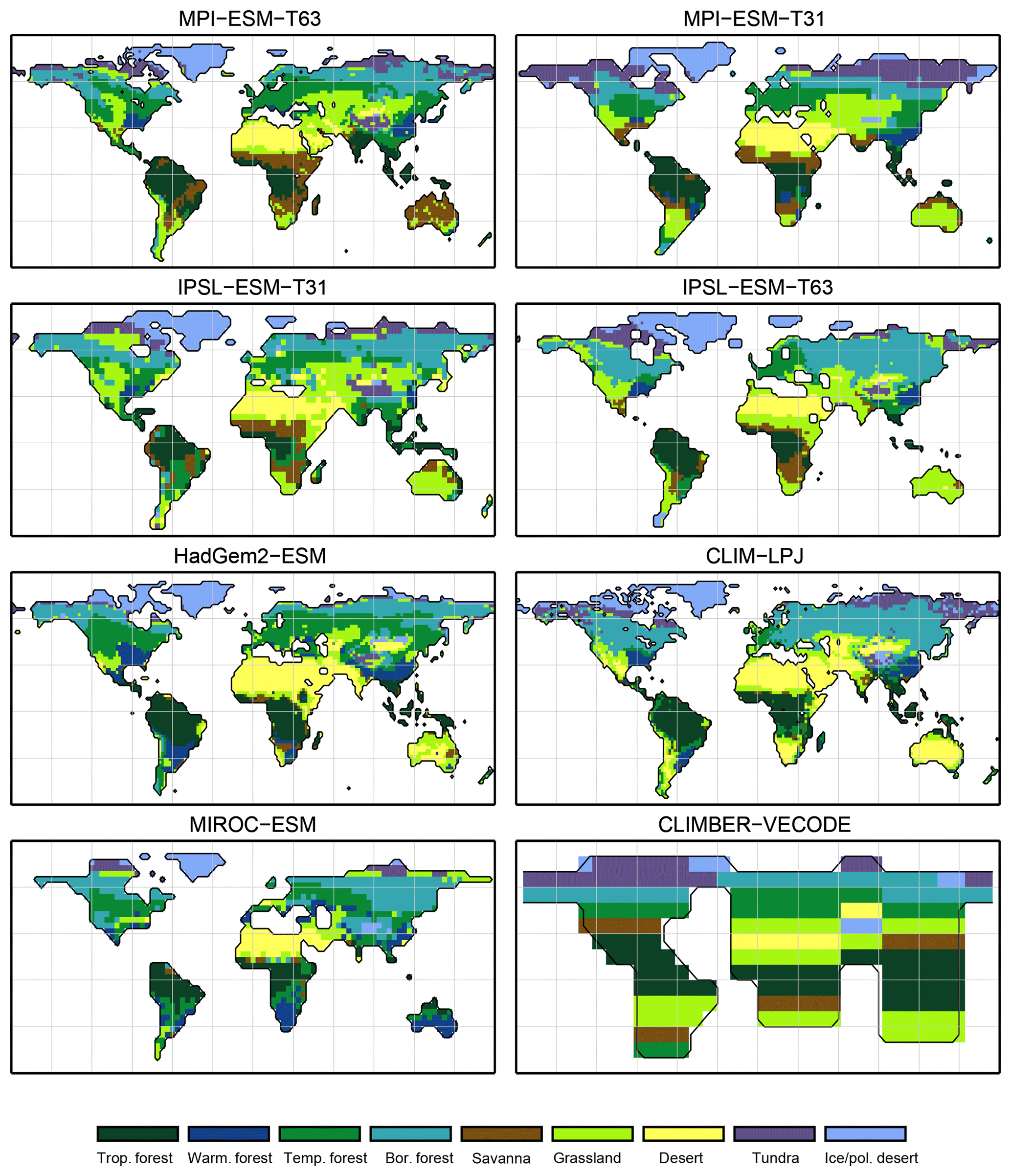
Figure 3Simulated pre-industrial mega-biome distributions according to the new biomisation method (PFT-based method). The PFT fractions simulated by the individual models have been converted into mega-biomes through climate limitation rules and assumptions on the maximum coverage of certain PFTs needed in the grid cells.
At this point it should be noted that we have selected the metrics in accordance with the research question of this study. For other purposes, such as estimating changes in biome distribution between present and future climate states, other metrics may be more appropriate, such as the Delta-V method, which also weights changes in vegetation attributes (Sykes et al., 1999). The metrics used in our study do not differentiate how far the biomes deviate in their properties; e.g. differences between tropical forest and tundra are equated as being qualitatively the same as differences between temperate and boreal forest.
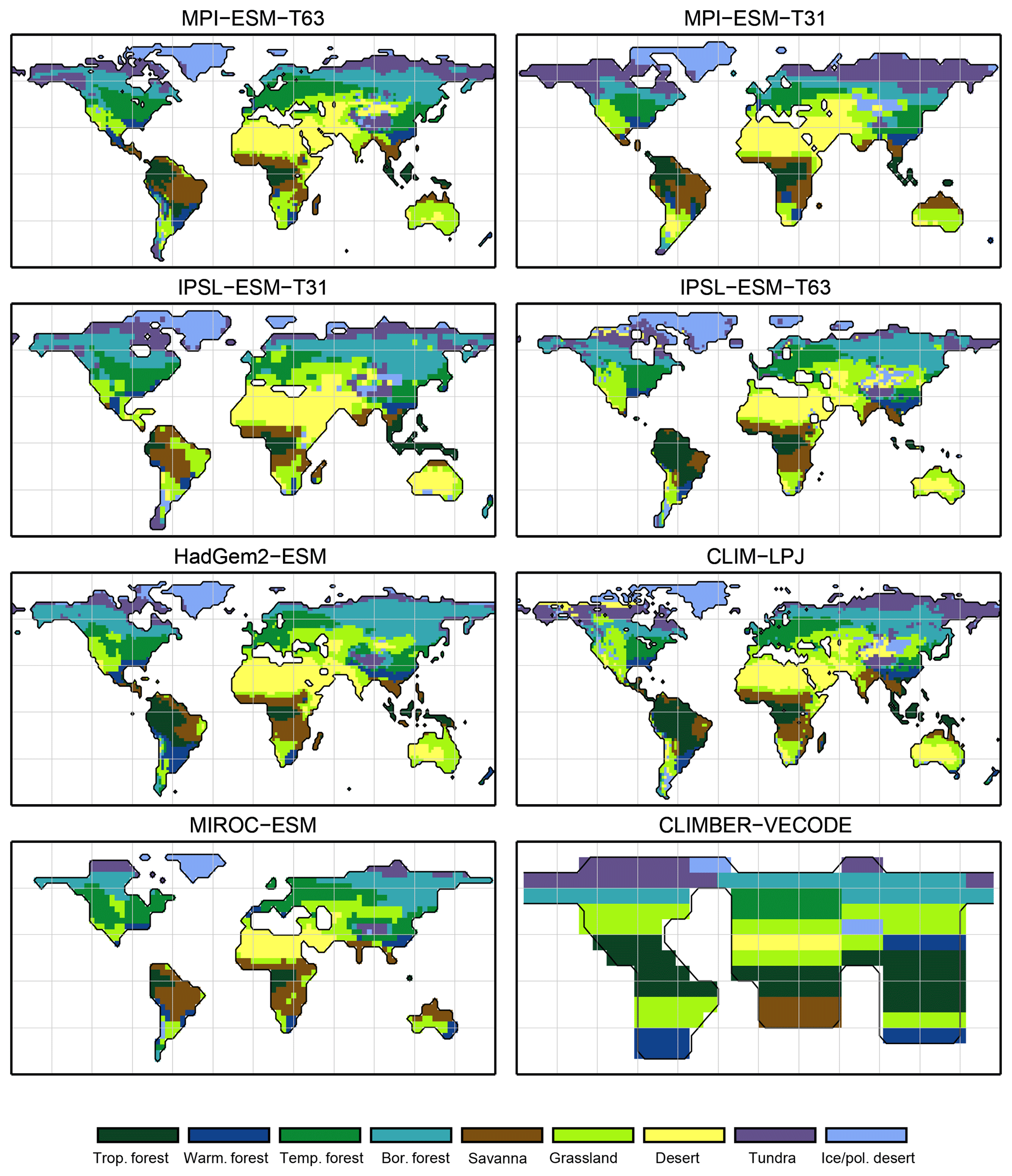
Figure 4Simulated pre-industrial biome distributions according to the classical biomisation approach, i.e. biomising the climate states simulated by the individual models. The climate field were used to force the biome model BIOME1 (Prentice et al., 1992). Afterwards, the original BIOME1 biomes were aggregated into the nine mega-biomes used in this study.
3.1 Comparison of the PFT-based and climate-based biome distributions for the pre-industrial time slice
For the pre-industrial time slice, the PFT coverage of eight different Earth system model simulations has been converted into mega-biome distributions (Fig. 3). Additionally, the underlying pre-industrial climate states are used as forcing for the BIOME1 model (i.e. the classical way of biomisation) to calculate the mega-biome distributions in equilibrium with the simulated climate states (Fig. 4). Overall, the PFT-based biome maps look similar to the climate-based ones. All major biome belts can be reproduced using the new method, independent of the resolution or the complexity of the vegetation models. The biomisation based on the PFT coverage generally assigns more grid cells to forest or woody biomes (e.g. savanna instead of grassland or desert) than the classical method. This is most noticeable in South America, where the area covered by tropical forests is strongly increased in the PFT-based biome distribution (Table D1), being more in line with observations. Likewise, the savanna and/or forest biomes are more spread out on the African continent for nearly all biomisations with the exception of the CLIMate-BiosphERe 2 (CLIMBER-2) model and IPSL-ESM-T63.
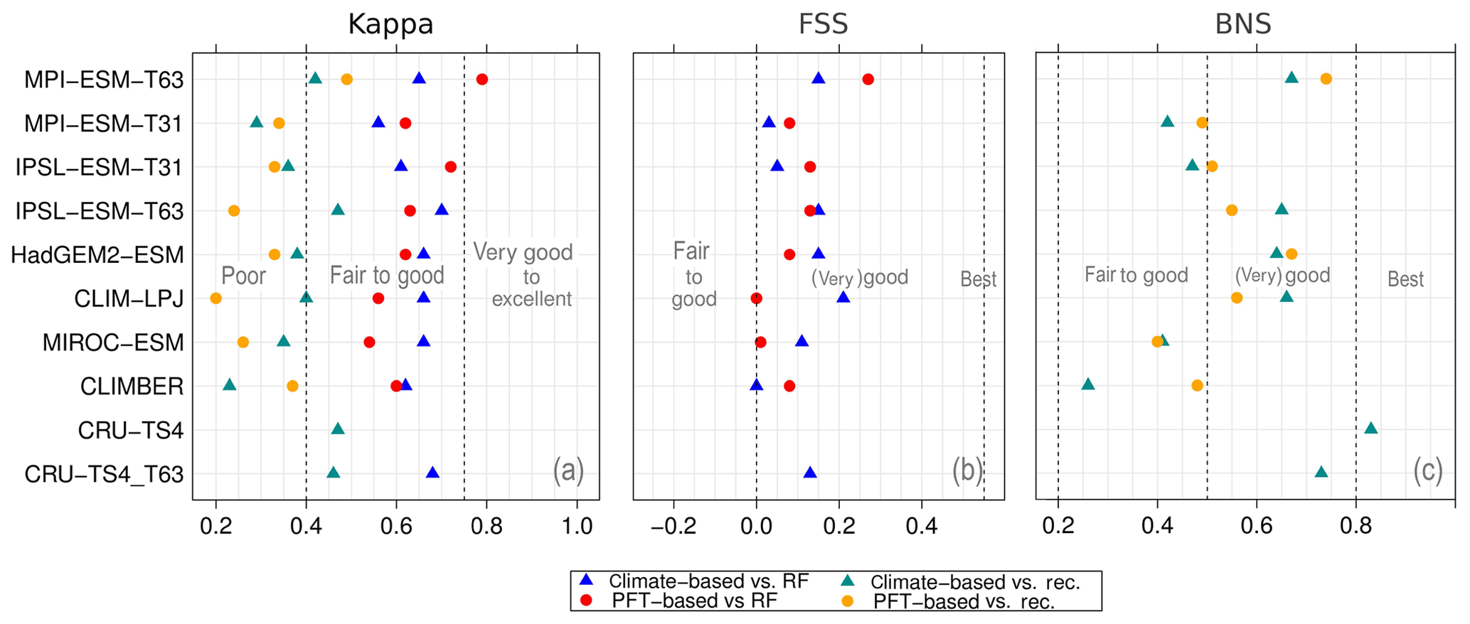
Figure 5Metrics quantifying the total agreement of the simulated pre-industrial biome maps based on the PFT cover fractions (PFT method) or based on the climate state (classical approach using BIOME1) with the reference datasets, i.e. modern potential natural vegetation (RF) and pre-industrial pollen-based biome reconstructions (rec.). Shown are the kappa values (a), the relative fractional skill score (FSS, b) and the best neighbour score (BNS, c) for all models and also for the biomisation based on the CRU TS4 observational climate data in original resolution (CRU TS4) and interpolated to a T63 grid (CRU TS4_T63).
The Asian forest regions are slightly larger in most PFT-based biome distributions compared to the climate-based ones. This impression is reinforced by the fact that for CLIM-LPJ and IPSL-ESM-T63 the PFT method suggests a pronounced boreal forest belt in northern Asia, not only reducing the size of the grassland but also that of the temperate forest area.
For North America, the PFT-based approach yields less forest for MPI-ESM-T63 and IPSL-ESM-T31 than shown by the climate-based biomisation. As a consequence, the North American prairie fits better to observations for the PFT-based biome distributions. In Alaska and north-western Canada, parts of the tundra regions suggested by BIOME1 tend to be replaced by boreal forest when using the new approach, which is generally more consistent with the observed vegetation.
The differences between the PFT-based and climate-based biome distributions can be caused by deficiencies in the biomisation methods, biases related to the imperfect vegetation models or biases in the simulated climate. While the effect of shortcomings in the vegetation models cannot be disentangled, the caveats of the PFT-based method and the effect of climate biases on the PFT-to-biome conversion are further discussed in Sect. 4.
3.2 Quantitative comparison of the PFT-based biome distributions with reference biome maps
To quantify the skill of the new method to represent the global biome distribution, we compare the resulting biome maps with the modern potential natural vegetation cover estimated by Ramankutty and Foley (1999, RF99 in the following) and the pre-industrial biome reconstructions provided by the Biome6000 project (Harrison, 2017). As target for the skill, the level of agreement between the BIOME1 derived biome distribution of the observed climate (CRU TS4, 1901–1930; cf. Fig. 2) and the reference datasets is taken, i.e. κ of 0.68 and FSS of 0.13 (Fig. 5) with respect to RF99 and a κ of 0.46 and BNS of 0.73 with respect to the biome reconstructions.
The PFT-based biome distributions agree well with the references, independent of the model. The kappa statistic shows an overall agreement to RF99 between 0.54 (for MIROC-ESM) and 0.79 (for MPI-ESM-T63) revealing a good to very good agreement (Fig. 5). Likewise, all models reach in total the level of good skill in the FSS metric (0.01–0.27). This agreement is in line with or even better than the match between RF99 and the climate-based biomisation and that between RF99 and the CRU TS4 biomisation that is taken as the target skill (Fig. 5). However, the spread between the individual models is larger for the PFT-based method than for the classical approach.
As expected, the kappa statistic indicates that the PFT-based biome maps compare worse with the reconstructions than with RF99, underestimating the similarity to the point reconstructions. κ ranges from 0.2 (poor) to 0.49 (fair), which is in line with the target skill and the metrics for the climate-based biome maps. The BNS, additionally considering accordance in the neighbouring grid cells of the record sites, reveals a good to very good agreement of the PFT-based biome distributions and the records (between 0.40 and 0.74), not much lower than the target skill and in accordance with the climate-based biomisations. For the MPI-ESM, IPSL-ESM-T31, HadGEM2-ESM and CLIMBER biomisations, the PFT-based method even produces biome distributions that fit better to the biome reconstructions than the climate-based biome maps.
Despite the overall agreement between the PFT-based biome distributions and the references, a closer look at the representation of individual mega-biomes in the converted maps indicates large differences among the models as well as among the individual mega-biomes (Fig. 6). While tropical forests and deserts compare best with RF99, the biome “warm–temperate forest” is not reproduced, independent of the underlying model simulation.
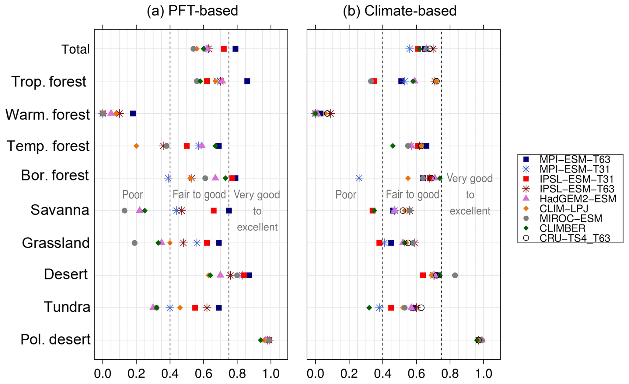
Figure 6Kappa metric quantifying the agreement of the simulated pre-industrial individual mega-biomes with the reference dataset (i.e. modern potential natural vegetation) for the PFT-based method (a) and the classical method using BIOME1 forced with the simulated background climate states (b).
The skill for simulating the other biomes is very different for the diverse models. κ spreads from poor for one model to very good for other models. Correcting the PFT distribution in land-use areas by redistributing the area fraction to the other tiles has no impact on the performance of the method. The biome maps based on simulations applying land use do not compare worse with RF99 than the maps of other simulations. Likewise, the complexity of the vegetation model and the number of distinguished PFTs have no significant effect on the representation of the biome distribution, indicating that the climate limits used in the biomisation procedure are appropriate for the assignment of the PFTs to the distinct PFT groups. The differentiation of the PFT types (e.g. the different forest types) in vegetation models is often based on similar climate limits, regardless of whether the model is a complex dynamic vegetation model or a simple biome model. With the exception of the PFT-based biomisation for CLIMBER, in which the coarse grid is clearly disadvantageous for capturing the reconstructed desert belts and the rather regionally confined biomes (savanna, warm–temperate forest), the spatial resolution of the models is not the primary factor for the spread in the metrics. The PFT-based method performs equally well for simulations using T63 as for simulations using T31 (in total); only the regionally distributed warm–temperate forest is better represented in finer resolutions.
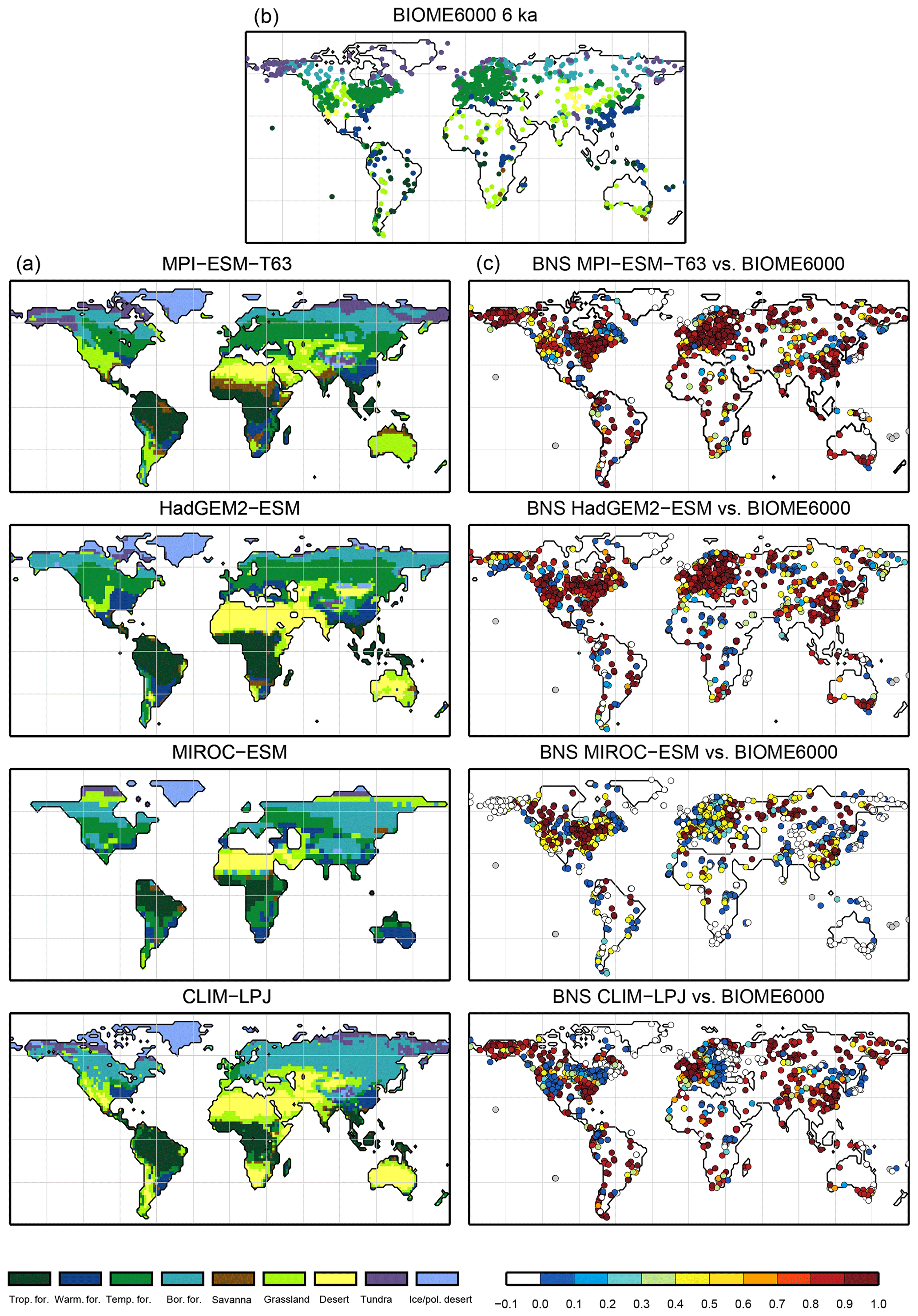
Figure 7Simulated mid-Holocene biome distribution in the different models, based on the PFT method (a), pollen-based biome reconstructions of the mid-Holocene biome distribution (BIOME6000 database, b) and the best neighbour score (BNS) for all individual sites showing the agreement of the reconstructed biomes and the biome distribution in the neighbourhood of the sites, ranging from 0 (no grid cell in the surrounding area shows the same biome as reconstructed) to 1 (the grid cell locating the site and the record at the site indicate the same biome) (c).
In general, the skill in representing the individual mega-biomes is similar for the PFT- and climate-based methods. Both approaches have the same strengths and weaknesses, but the spread between the models is larger for the PFT-based biomisations. In comparison to the climate-based method, the tropical, the warm–temperate and the boreal forest biomes tend to be slightly better represented by the PFT-based method. In contrast, the temperate forest, savanna and grassland distribution – averaged over all models – fit better to RF99 when using the climate-based approach, although for individual simulations, κ derived for the PFT biomisation exceeds the climate-based one. The savanna and grassland biomes are particularly misrepresented in the biome maps that are based on the PFT distributions simulated by MIROC-ESM, CLIMBER, CLIM-LPJ and HadGEM2-ESM. The temperate forest is poorly reproduced only in the PFT-based biomisation of CLIM-LPJ. Overall, the metrics indicate that the PFT-based method works as well as the classical approach of biomising climate states via the BIOME1 model. Likewise, the method is able to keep up with the method by Prentice et al. (2011), further discussed in Appendix E.
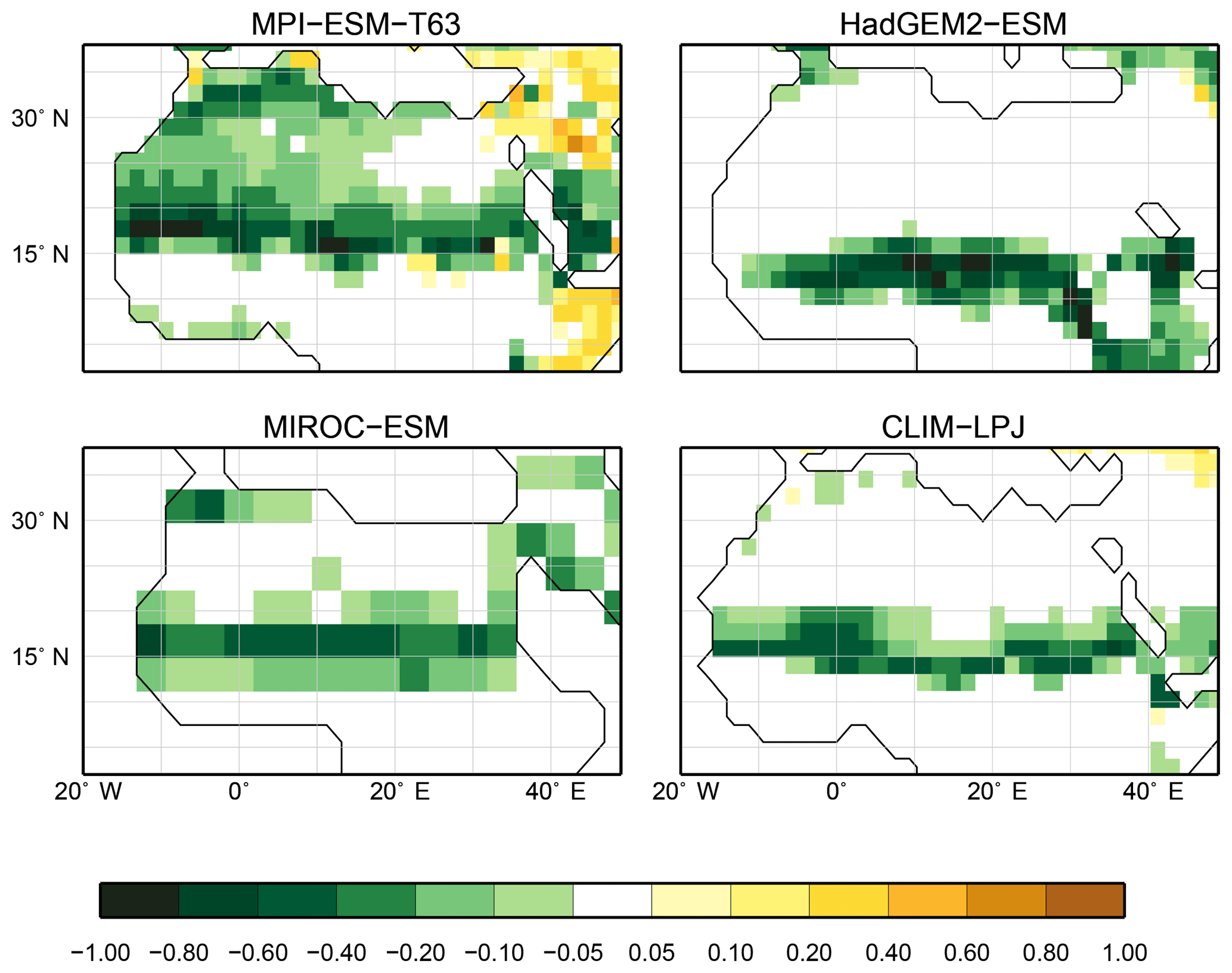
Figure 8Differences in the desert fractional coverage simulated by the individual models between the mid-Holocene (6 ka) and pre-industrial time slices (0 ka).
3.3 PFT-based biome distributions for the mid-Holocene and Last Glacial Maximum time slice
The sensitivity of the PFT-based method to changes in the vegetation cover is assessed by evaluating palaeo-biome distributions. For the mid-Holocene time slice, four different simulations have been analysed. The main vegetation changes described by biome reconstructions are the northern shift of the Northern Hemisphere forest belts, in particular a northward displacement of the taiga–tundra boundary, and the decrease of the desert areas compared to pre-industrial time slice. According to the BIOME6000 records, grassy vegetation reached at least up to 26∘ N at 6 ka, far into the modern central Sahara (Fig. 7). For none of the models is this biome shift reproduced, neither in the PFT-based (Fig. 7) nor in the climate-based biome distributions (not shown). The mean Sahara desert border shifts northward by one to two grid cells in the biomisations (i.e. approximately 1.875 to 3.75∘, Table 4). This shift collocates with substantial reductions in the desert fractions simulated by the individual ESMs (Fig. 8). Only in MPI-ESM-T63 is vegetation increased in the entire western and central Sahara, but this increase is lower than 20 %, not leading to a change in the biome assignment from desert to grassland. As the climate-based biomisations performed with BIOME1 reveal a reduction of the Sahara desert area in the same magnitude as the PFT-based ones, we conclude that the new biomisation method shows a reasonable sensitivity to the simulated changes in the desert fractions.
For all models with the exception of MIROC-ESM, the PFT-based biomisation reproduces an increased forest biome fraction in Eurasia north of 60∘ N during the mid-Holocene compared to pre-industrial time slice, in line with the biome reconstructions (Table 5). However, the magnitude of the change differs between the models, ranging from 0 % within MIROC-ESM to 12 % within CLIM-LPJ. For nearly all models (except for MIROC-ESM), the expansion of the forested area in the high northern latitudes seen in the PFT biomisation is of similar magnitude to that in the climate-based biomisation, confirming that the method covers past vegetation changes with reasonable sensitivity.
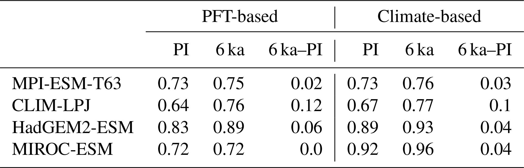
Table 4Position of the desert margin (∘ latitude) in north Africa at PI and 6 ka and the differences in position of the desert margin between 6 ka and PI (∘ latitude), for the PFT-based biomisations and the climate-based biomisations. The desert margin is here defined as latitude at which the zonal mean desert biome fraction averaged over the region 15∘ W to 30∘ E exceeds 50 %.
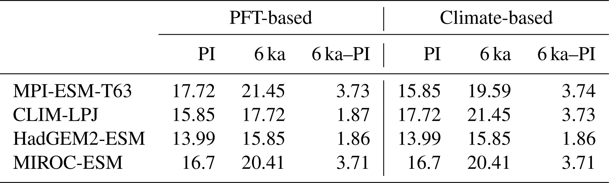
Table 5Mean forest biome fraction in northern Eurasia (60–80∘ N, 0–150∘ E) in the PFT-based biomisations and the climate-based biomisations for the mid-Holocene (6 ka) and pre-industrial (PI) time slice, and the difference between both (6 ka–PI).
Overall, the biome distributions for the mid-Holocene compare equally well to the reconstruction as they do for the pre-industrial time slice (Fig. 9). Although κ is similarly low, ranging from 0.17 for the CLIM-LPJ biomisation to 0.38 for the MPI-ESM-T63 biomisation (poor agreement), the spread in the models and the differences in κ between the PFT-based biomisations and the climate-based biomisations is nearly identical to the results for the pre-industrial biome distributions. In line with the results for PI, the BNS indicates a good to very good agreement to the biome reconstructions (ranging from 0.44 for MIROC-ESM to 0.72 for MPI-ESM-T63). The skill to capture the reconstructed individual mega-biomes strongly depends on the number of available pollen records; thus, temperate and boreal forests are represented best (Fig. 7), while the simulated savanna regions are not supported by the biome reconstructions.
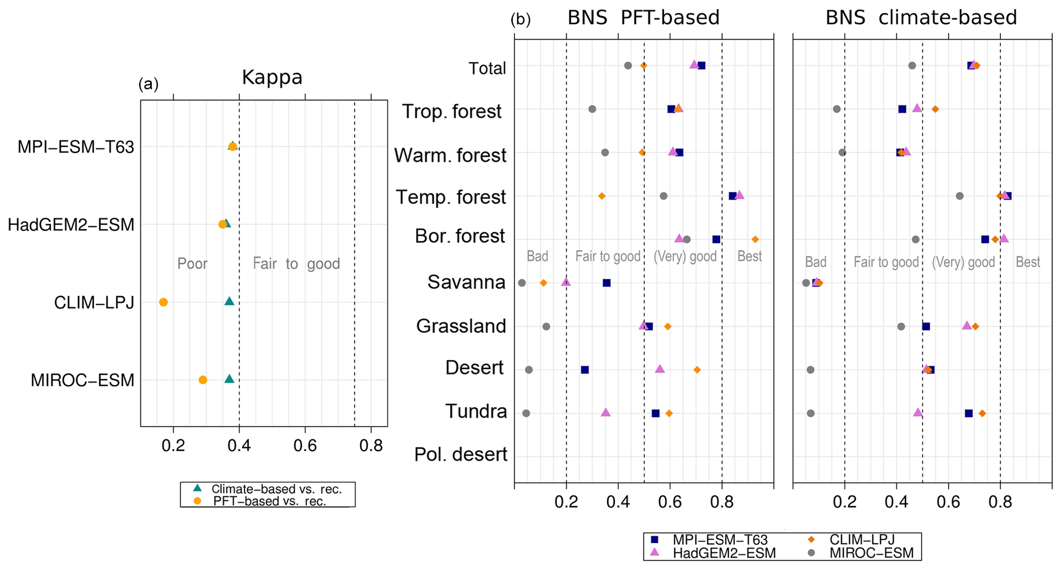
Figure 9Metrics quantifying the agreement of the simulated mid-Holocene biome maps based on the PFT method or based on the climate states (i.e. according to the BIOME1 model) with the pollen-based biome reconstructions (BIOME6000 database) for the mid-Holocene time slice, i.e. the (total) kappa value (left panel) and the BNS values for the individual mega-biomes.
For the Last Glacial Maximum time slice, five different simulations have been analysed. According to BIOME6000, the main reconstructed vegetation differences at LGM compared to PI are a strong equatorward retreat of the forest biomes and an expansion of tundra and steppe regions. The northernmost record indicating boreal forest during LGM is located at approximately 51∘ N in Asia (Fig. 10). The PFT biomisations mostly reproduce this reduction and the shift in Northern Hemisphere forest biomes (Fig. 10), though the extent of the shift is underestimated. Forest reaches up to 50∘ N (for CLIMBER) to 65∘ N (for MPI-ESM-T63). The boreal forest position in the MIROC-ESM biomisation is not much changed compared to PI, but the boreal forest nearly replaces the temperate forest biome.
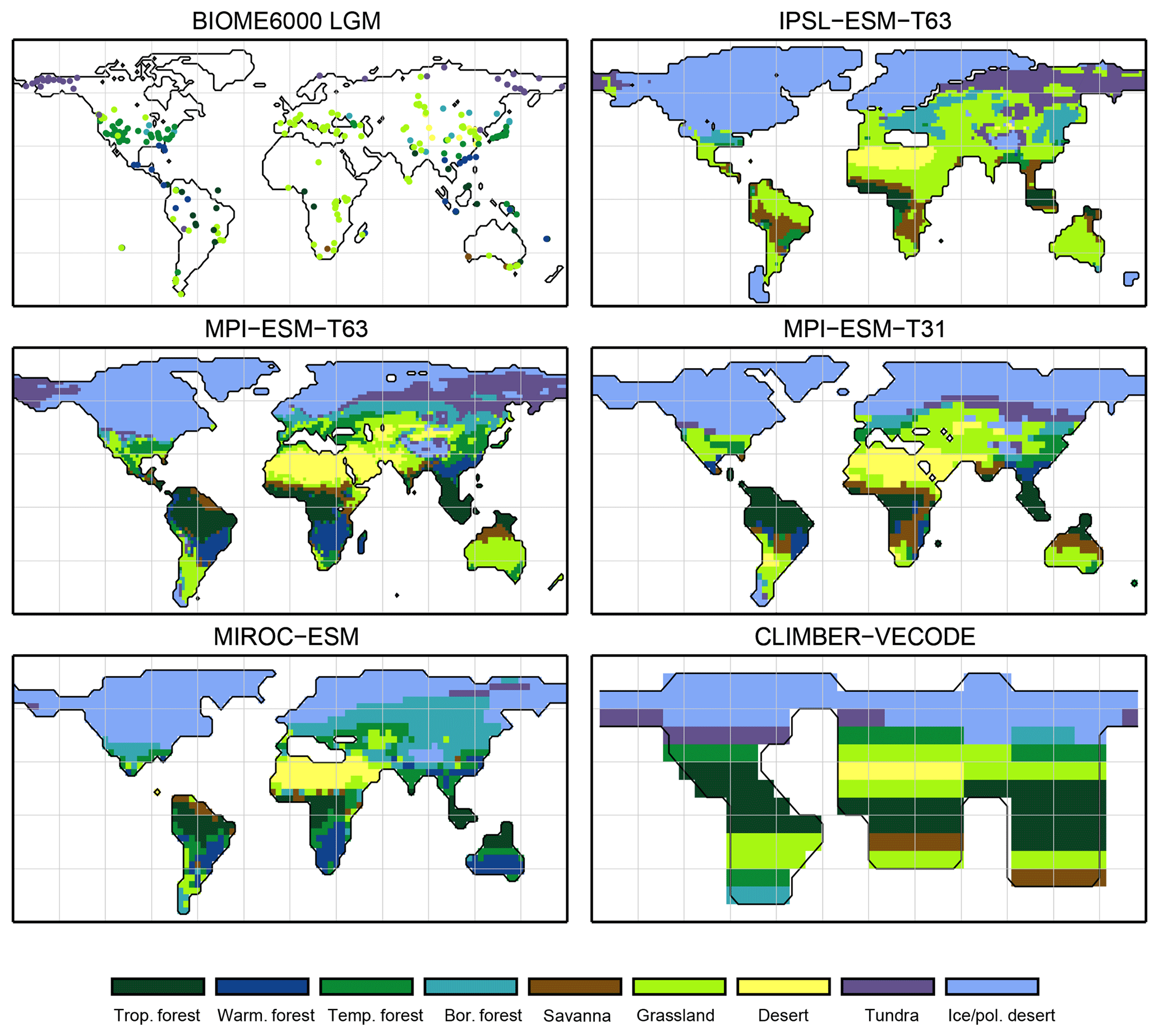
Figure 10Pollen-based biome reconstructions (BIOME6000 database) for the Last Glacial Maximum time slice and the simulated biome distributions according to the new biomisation method (i.e. the PFT-based method).
The overall agreement of the PFT-based biome distributions with the biome reconstructions is rather fair but in line with the results for the climate-based biome distributions. κ ranges from 0.07 for MPI-ESM-T31 to 0.23 for CLIMBER, only indicating a poor similarity of the biome maps and records (Fig. 11). The BNS ranges from 0.24 (for MIROC-ESM) to 0.57 (for MPI-ESM-T63) revealing a fair to good agreement. The values for both metrics are in the same magnitude as for the climate-based biomisations. Similar to the PI time slice, neither the complexity nor the spatial resolution is the main reason for the differences between the PFT biomisations. The spread in the skill of representing the individual biomes is large, and no systematic bias for one model can be found. With the exception of the biomisation for CLIMBER, the savanna biome is misrepresented in all biomisations, independent of whether the PFT-based or the climate-based method was used. Within the model ensemble, tropical and temperate forest can be reproduced best.
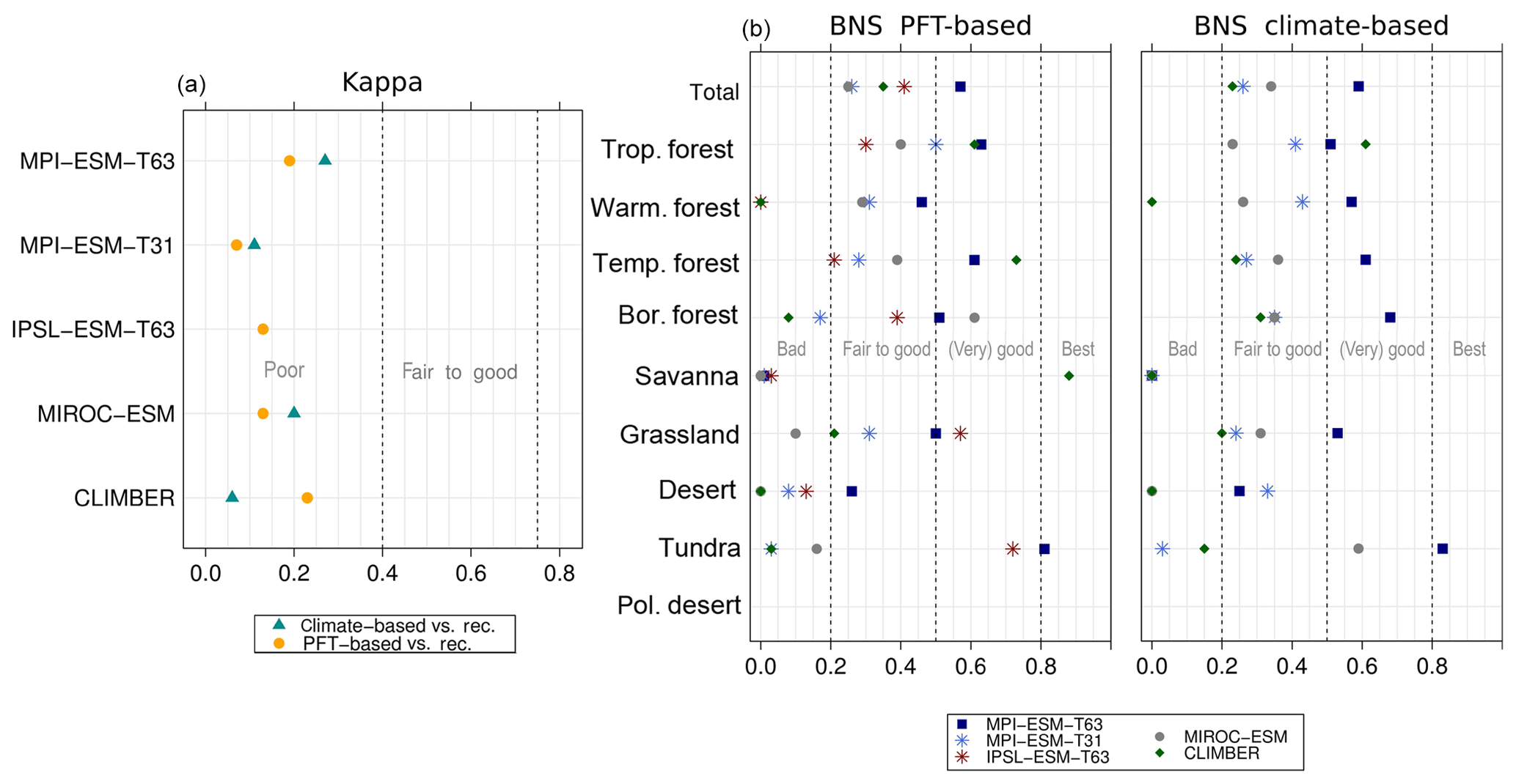
Figure 11Metrics quantifying the agreement of the simulated Last Glacial Maximum biome maps based on the PFT method or based on the simulated climate states (i.e. according to BIOME1) with pollen-based biome reconstructions (BIOME6000 database), i.e. the (total) kappa value and the BNS values for the individual mega-biomes. Please notice that the climatic variables needed to force BIOME1 could not be provided for IPSL-ESM-T63. Thus, no climate-based biomisation exists for IPSL-ESM-T63.
4.1 Caveats in the method
Even if the biomisation is restricted to mega-biome level, no clear definitions exist to distinguish biomes in terms of plant functional type compositions. While the bioclimatic limits used in the biome models are based on empirical analysis, no equivalent classification regulates the biomisation of PFTs. We particularly face this problem in finding a meaningful threshold of maximum tree cover needed for defining forests. When is an accumulation of trees identified as forest? As models tend to underestimate the forest coverage and forest extent in the high northern latitudes (cf. Loranty et al., 2013), we choose the assumption of tree cover being just dominant in forested grid cells, although this limit is very low. We test other limits (e.g. absolute dominance, i.e. fractional coverage exceeding 50 %), but these work worse for most simulations used in this study as well as for other simulations.
The mega-biome “warm–temperate forest” (e.g. subtropical forest) includes PFTs that can be assigned to several biomes and is rather defined by a coexistence of certain PFTs. For instance, in the BIOME4 model, it is not only defined by the dominance of temperate evergreen broadleaved trees but can also be defined by a dominance of cool conifers (with a sub-PFT of temperate evergreen broadleaved trees). The cool conifers – in turn – are also part of temperate forest biomes. Given the limited number of PFTs in the DGVMs, the confinement of biomes via PFT mixtures is not possible. As biome models such as BIOME4 generally manage to simulate warm–temperate forests at the correct locations, we adopt the bioclimatic limits from BIOME4 (limit for temperate evergreen broadleaved trees) for defining this mega-biome. Nevertheless, the calculated warm–temperate forest distribution strongly disagrees with the reference datasets. The reconstructed biome “warm–temperate forest” shares some subtropical PFTs with the tropical evergreen forest (Ni et al., 2010). These biomes are quite different in key species, but not on genus or family level, on which the pollen identification in the reconstructions is performed. Thus, these biomes tend to overlap in some regions and are sometimes mixed up in reconstructions (Chen et al., 2010). In addition, this mega-biome includes the warm–temperate rainforest and the wet sclerophyll forest and woodland in the BIOME6000 reconstructions (cf. Harrison, 2017), which may not be able to be identified with our biomisation method. Regarding the modern reference of RF99, we decided to assign the biome “temperate needleleaf evergreen forest and woodland” of the RF99 dataset to the mega-biome “temperate forest”, although this biome is also located, e.g. in the southern US, which should be assigned to the warm–temperate forest. Therefore, the evaluation of this method with respect to warm–temperate forest might be ambiguous. Furthermore, warm–temperate forests are small and rather patchily distributed and are thus rarely dominant in the coarse grid cells to which the RF99 reference had to be interpolated to. The coarser the grid is, the more warm–temperate forest regions get lost during the interpolation. Therefore, the warm–temperate forest biome is generally better represented for models using a higher spatial resolution (i.e. MPI-ESM-T63, CLIM-LPJ and IPSL-ESM-T63).
In addition, not all biomes can be differentiated by the structural composition or climatic tolerance. The biome “savanna” is the second-largest ecosystem in the tropics, covering approximately one-fifth of the global land surface (Scholes and Hall, 1996). It occurs in climatic zones that are also suitable for forest and grasslands (Lehmann et al., 2011) and is thus very variable regarding the plant composition. Tree fraction can vary from very dense (open forest savanna) to nearly zero (Torello-Raventos et al., 2013). While tropical savannas require the coexistence of trees and C4 grass, they can only be distinguished from forests by their unique functional ecology, fire tolerance and shade intolerance (Ratnam et al., 2011). These features make savannas unstable and vulnerable to changes in, e.g. grazing, fire regime and climate, transforming savannas into forest or grasslands (Franco et al., 2014). The functional diversity of savannas is not adequately included in DGVMs nor considered in the biomisation method presented here. As even C4 grass is not simulated in all models, we had to define the savanna biome in a very rudimentary manner by a mixture of woody PFTs and grass and by bioclimatic limits, i.e. a mean temperature of the coldest month exceeding 10∘ which is taken as a limit for C4 grass in dynamic vegetation models (e.g. Jena Scheme for Biosphere Atmosphere Coupling in Hamburg; JSBACH; cf. Reick et al., 2013). The savanna biome might therefore not be represented well. At least in the palaeo-simulations, most biomisations do not capture the reconstructed savanna area, but this may partly also be related to the fact that only few records exist indicating savanna during LGM and 6 ka. Modern pollen rain analysis reveals that woody plant taxa typically characterising savannas are underrepresented or even absent in the pollen/vegetation ratios. Given the lack of savanna indicators, this biome may be overlooked in fossil pollen records (Jones et al., 2011).
Similar to dynamic vegetation models, the priority in the biomisation procedure is given to forest biomes. It is first tested whether forest biomes are suitable for covering the grid cell, before the savanna is distributed. Grasslands and tundra are assigned to the residual grid cells, independent of the real grassy PFT cover fractions. The only restriction is a total vegetation coverage exceeding 10 % for tundra or 20 % for grassland to be distinguishable from deserts. This method has the large disadvantage that biases in the forest distribution propagate throughout the assignment of all biomes with the exception of deserts. The forest biome distribution calculated for the different models is further tested in Sect. 4.3 for the pre-industrial time slice.
Another problem is the inclusion of anthropogenic plant functional types (i.e. land use) in some simulations, making the biome distribution less comparable to the reference data. Although land use is often prescribed in the models, this process cannot be reversed in the final output data. The area chosen for land use is historically determined and is based on human decisions and not primarily on climate conditions. These human pathways cannot be reproduced in simple biomisation methods nor in the current dynamic vegetation models. We artificially rescale the natural vegetation in human-affected regions by redistributing the fraction of anthropogenic PFT coverage proportionally to the natural PFTs. This is a very simple approach and only partly in line with the implementation of land use in the dynamic vegetation models. For instance, within JSBACH, pasture is preferentially assigned to natural grasslands; forests are only affected if prescribed pasture fraction exceeds the natural grassland area (cf. Reick et al., 2013). This rule is plausible but not reversible and therefore not appropriate for the biomisation method presented here. The results show that biome maps based on models including land use do not agree worse with the references than the other simulations, underlining that the redistribution method used here provides a good approximation of the natural vegetation cover.
The method of PFT biomisation basically uses bioclimatic limits that have been inferred for the modern vegetation–climate relationships. These limits may not be valid for all time periods. During LGM, the atmospheric CO2 concentration was substantially lower than today, which may also affect the response of the plants to the background climate. Likewise, the matrices for the assignment of taxa into PFTs and from PFTs into biomes have been constructed on the basis of the recent vegetation. These matrices do not have to be constant in time; i.e. they may not be applicable for glacial vegetation. Furthermore, the classification of the biomes itself corresponds to the modern vegetation and does not necessarily have to reflect the palaeo-vegetation. There might be other biomes in glacial climates that remain unconsidered. This may lead to biases in the modelling results and the biome reconstructions taken as reference. The κ values for the LGM time slice were quite low, indicating disagreement between the simulated and reconstructed biome distributions.
A rather technical problem is the interpolation of the PFT distributions to the T31 or T63 grid that partly leads to a decrease in the global area to be compared with the reference datasets due to a mismatch of the land–sea masks. In regions with a strong change of the PFT fractional composition (e.g. desert border, coastal region), the interpolation may produce blurry transitions in the PFT distributions resulting in an erroneous conversion into the mega-biomes.
4.2 Biases in the pre-industrial biome distributions and the influence of the climate background
The classical method of biomising climate states via biome models (here BIOME1 by Prentice et al., 1992) and the new PFT-based method result in similar biome distributions for most models and all time slices. Generally, the PFT-based method produces more forest in comparison with the classical approach. This is mainly related to the rather low limit of forest fraction needed in the assignment of forest in the PFT-biomisation procedure. In forest regions, where Earth system models tend to produce large biases in the climate state, the PFT-based approach may be more suitable for the biomisation. Therefore, the tropical, warm–temperate and boreal forests are probably better represented by the PFT method. However, the biomisation of the PFT distributions itself strongly depends on the underlying climate, affecting both the differentiation into the biomes as well as the simulation of the PFT coverage in the different dynamic vegetation models. To accurately compare the performance and the skill of the different vegetation models to represent biome distributions, the models should therefore be forced by the same climate state, but only few models can be run offline. This study is thus not thought of as a model evaluation but as an introduction to the biomisation method and as a test of whether the procedure works for models of different complexity and simulations for different time slices.
To assess the contribution of the effect of biases in the underlying climate to the differences in the PFT-based biomisations and the references, we compare the pre-industrial climate-based biomisations with the biomisation of the CRU TS4 dataset. A sensitivity study is performed following Dallmeyer et al. (2017) to relate differences in the biome distributions to precipitation or temperature deviations in the background climate (Fig. 12). For this purpose, we successively replace the temperature or the precipitation in the CRU TS4 forcing file for the BIOME1 model with the respective pre-industrial temperature or precipitation distributions simulated by the models. Afterwards, we compare the differences between the calculated biome distributions.

Figure 12Climate factors leading to the differences between the pre-industrial climate-based biome distributions and the biome distribution inferred from the CRU TS4 observational climate data. The factors were calculated by performing a sensitivity test with the BIOME1 model following Dallmeyer et al. (2017) by successively replacing the temperature or the precipitation in the CRU TS4 forcing file for BIOME1 with the respective data from the different PI simulations.
Generally, disagreement in the high northern latitudes is associated with biases in temperature, while disagreement in low latitudes co-occurs with precipitation biases for the pre-industrial time slice. The similarity of the PFT biomisations and RF99 is lowest for CLIMBER, MIROC-ESM and CLIM-LPJ. While for CLIMBER the coarse resolution (i.e. the very different land–sea masks) may be the main responsible factor for disagreement, total κ is reduced by an underestimation of grasslands and savanna and an overestimation of the forests in the PFT-based biomisation of MIROC-ESM. This is exactly opposite to the biases occurring in the climate-based biomisation, indicating that the climate is not the primary origin of the differences. For this specific model, the PFT-based biomisation strongly differs from the climate-based one. This may at least partly be related to the handling of vegetation in the model. The spatially explicit individual-based (SEIB) vegetation model included in MIROC-ESM is a forest gap model, not using the tiling approach (Sato et al., 2007). PFT fractions have only been estimated during the CMIP5 post-processing, based on the net primary productivity ratios of the different vegetation categories. This approach might lead to an overestimation of forest. On the other hand, according to BIOME1, the underestimation of the tropical forest domain in the climate-based biomisation of MIROC-ESM is caused by the way to dry climate in South America.
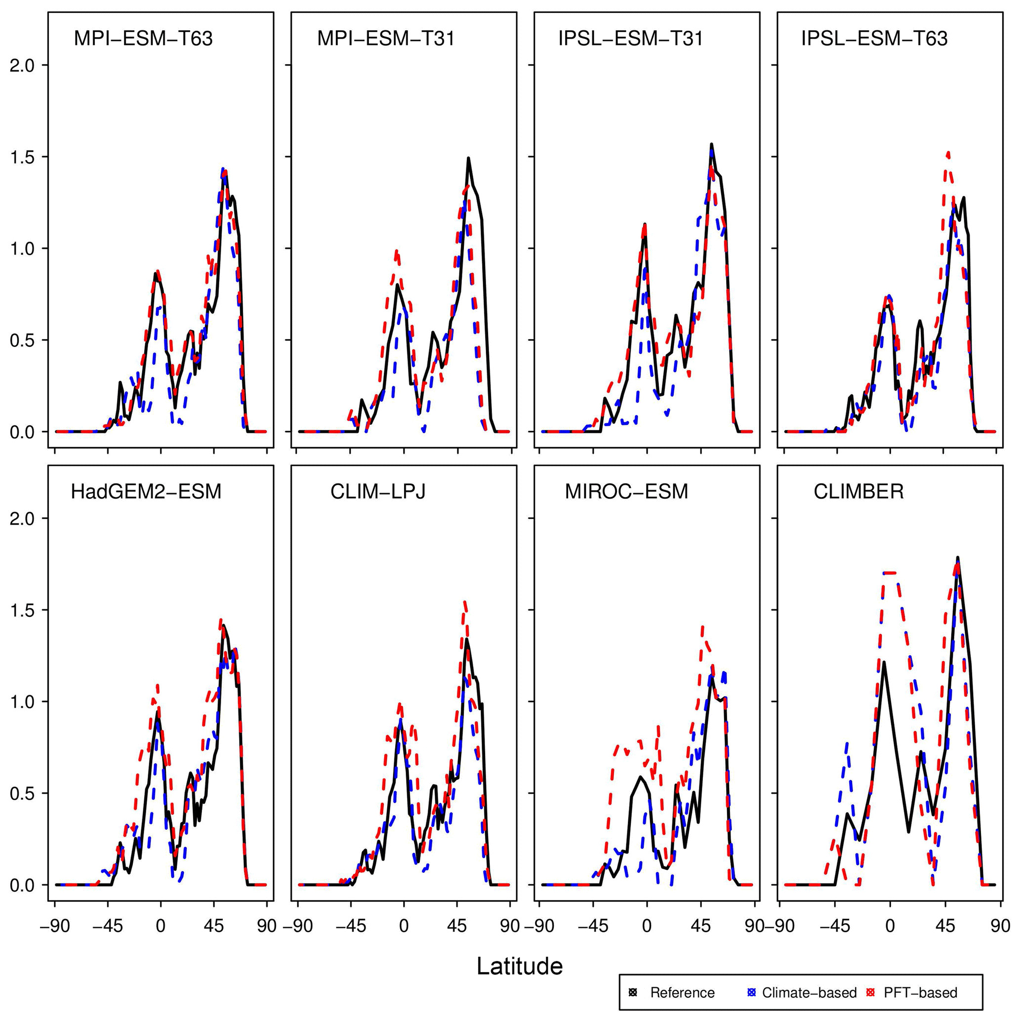
Figure 13Zonal sum of pre-industrial forest biome area per latitude (million km2 degree−1) in the reference (RF99), the climate-based biomisation (blue) and the PFT-based biomisation (red) for each of the individual models. Due to the special land–sea mask in CLIMBER, the values for this model have been scaled by a factor of 0.766, which is the quotient of the global land area in a Gaussian T31 grid and the global land area in the CLIMBER grid ().
In the PFT biomisation of CLIM-LPJ, κ is basically reduced by an overestimation of boreal forest at the expense of temperate forest and an underestimation of the savanna regions. Both errors are mainly not climate driven. Within dynamic vegetation models explicitly calculating boreal and temperate forest, these forest types can coexist. To give a clear assignment, we decided to differentiate both forest types by the dominant tree PFT, i.e. if the boreal tree fraction exceeds temperate tree fraction, forest fraction is assigned to boreal forest, and vice versa. This partly disagrees with the handling in biome models; e.g. in cool mixed forest, boreal trees could be the dominant PFT and temperate trees only the subdominant PFT (cf. Kaplan et al., 2003), but this biome would be assigned to the mega-biome “temperate forest”. We assume that due to a slight overestimation of boreal forest coverage in Europe and at the modern boreal to temperate forest transition zone within CLIM-LPJ, the vegetation in these regions is grouped into the mega-biome “boreal forest”. In South America, tropical forest fraction is overestimated by CLIM-LPJ, with values exceeding 80 % in most regions of Brazil, precluding the savanna biome. Within north Africa, CLIM-LPJ simulates hardly any regions with coexisting substantial forest and grass fractions. Either tropical trees are clearly the dominant PFT (assigned to tropical forest) or forest fraction is too low (below 10 %) to be assigned to savanna. The defined limits for savanna are only fulfilled for very few grid cells.
For MPI-ESM-T31, the boreal forest biome is strongly underestimated in the PFT-based biomisation. The BIOME1 results clearly relate this bias to a too-cold climate (GDD5 limit is not reached in BIOME1), which also affects the simulation of trees in JSBACH sharing the same bioclimate limits. Therefore, forest fraction in MPI-ESM-T31 is underestimated for the northern latitudes.
IPSL-ESM-T31 shows a dry bias in South America resulting in a too-low tropical forest biome cover in both the climate-based and the PFT-based biomisations. BIOME1 reveals another systematic bias for the MIROC-ESM biomisation indicating too much temperate forest in North America at the expense of grassland and partly of boreal forests. This overestimation of temperate forest is induced by a too-wet climate favouring growing of trees and a rather too-warm climate in the high northern latitudes.
4.3 Evaluating the distribution of forest biomes
Due to the forest priority rule in the biomisation method, the skill of representing the non-forested biomes depends on how well the forest distribution can be reproduced. To further assess the performance of the method with respect to the forest biomisation, we analyse the pre-industrial zonal mean forest fraction in the form of the zonal sum of forested area per latitude to be independent of the different grid sizes used for the individual simulations (Fig. 13). In nearly all PFT biomisations, the zonal forest fraction is underestimated in the high northern latitudes and the zonal maximum is shifted southward, although the defined limit of minimum required tree fraction is already quite low in the PFT method. This bias is most obvious in the biomisation for MPI-ESM-T31 and IPSL-ESM-T63. While for MPI-ESM-T31, the coexistence of the bias in both the climate-based and the PFT-based biomisations underlines the effect of the too-cold climate on the forest distribution, the strongly shifted high-latitude forest maximum in the IPSL-ESM-T63 PFT biomisation is probably not climate driven.
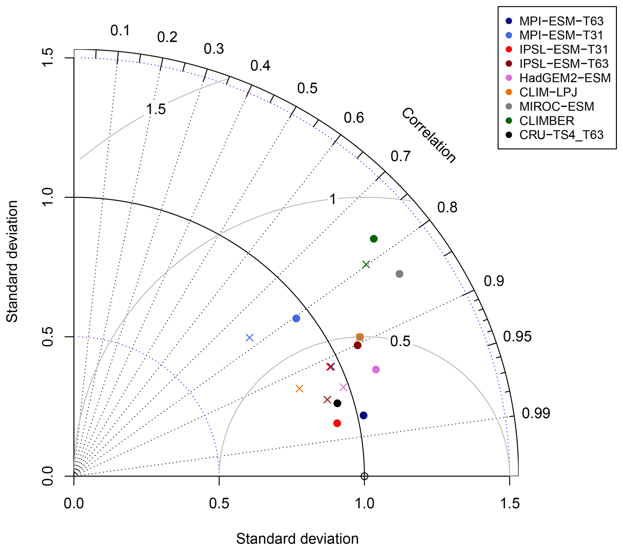
Figure 14Normalised Taylor diagram showing the agreement of the simulated pre-industrial zonal sum of forest biome area per latitude using BIOME1 (i.e. based on the simulated climate states; crosses) or the PFT-based method (dots) for the individual models with the modern potential biome distributions according to Ramakutty and Foley (1999, RF99). Additionally shown is the agreement of the CRU TS4-based biomisation with this RF99 reference dataset.
In the tropical regions, the forest fraction tends to be underestimated when using the climate-based method, whereas forest fraction is often too high in the PFT-based biomisations, probably related to the low tree fraction limit needed for forest assignment in the PFT method. The tropical forest fraction based on the simulated climate and PFT distribution by CLIMBER is strongly overestimated. This is at least partly caused by the coarse grid and specific land–sea mask used in the model.
To further quantify the biases in forest fraction, we compare the centred root mean square error (cRMSE), the Pearson correlation coefficient (r) and the zonal variability between the biomisations of the ESM simulations and the RF99 reference, combined in a Taylor diagram (Fig. 14). Overall, the zonal forest fraction in the biomisations agrees well with the reference. All biomisations show a good to nearly perfect pattern correlation with values exceeding 0.77, independent of the chosen method. For most models, the Pearson correlation coefficient even exceeds 0.9. The PFT-based biomisation is worst for CLIMBER and MIROC-ESM, revealing a too-large standard deviation and a cRMSE of 0.83 and 0.73, respectively. For MPI-ESM-T31, spatial variability is slightly too low and the cRMSE is 0.61 using the PFT-based method and 0.63 in the climate-based biomisation, reflecting the common underestimation of the boreal forest. As expected, best performance can be observed for the biomisations based on simulations with prescribed PFT coverage (MPI-ESM-T63 and IPSL-ESM-T31), sharing a similar standard deviation with RF99, a pattern correlation coefficient of 0.98 and a cRMSE of 0.21, which is even better than the biomisation of the CRU TS4 data (cRMSE of 0.28).
Dynamic global vegetation models use different kinds and numbers of plant functional types to represent the global vegetation. These PFT distributions can neither be directly compared between different models nor between models and reconstructions, which were hitherto mostly provided in the form of biomes. We have therefore developed a method for biomising simulated PFT distributions and have tested this method for six state-of-the-art dynamic global vegetation models based on simulations for the pre-industrial, mid-Holocene and Last Glacial Maximum time slices.
Overall, the method works well for all models and can keep up with other biomisation techniques. The comparison with different reference datasets (i.e. pollen-based biome reconstructions and estimates of the potential natural vegetation) reveals a similar agreement with the PFT-based biomisation than with biome distributions inferred from the biome model BIOME1 (Prentice, 1992) that has been forced with the background climates. The comparable skill to the BIOME1 model, which is tuned to represent the global vegetation as well as possible, is partly achieved by the use of bioclimatic limits that are in line with the definitions in biome models.
The skill of capturing the global biome distributions is independent of the spatial resolution and the complexity of the vegetation models or the integration of land use. For models just using two different PFTs (CLIMBER) the method performs equally well as for models using 10 different PFTs (e.g. IPSL-ESM). Only the very coarse resolution in the CLIMBER model hampers the comparability with the single point reconstructions, in particular for biomes with a very limited number of available records. In addition, the quantitative comparison of the biomised vegetation distributions among each other and with the gridded reference data is complicated by the very different model resolutions.
In general, large biome belts (such as tropical forest) can be captured best, while rather regionally confined biomes such as savanna and warm–temperate forest are not as well represented. This may at least partly be related to the fact that these biomes cannot be defined clearly via PFT cover fractions. Savannas are characterised by a distinct functional ecology and cannot be differentiated from other tropical biomes via plant composition or climatic tolerance. The warm–temperate forest is rather defined by a coexistence of PFTs and might overlap with other biomes. This may lead to mismatches with the reconstructions. For the palaeo-simulations, the agreement between the individual mega-biome distributions derived by the PFT method and the biome reconstructions strongly depends on the number of available records. The main vegetation differences between the pre-industrial and mid-Holocene or Last Glacial Maximum time slices are captured by most models and are also reflected in the PFT- and climate-based biomisations, indicating a reasonable sensitivity of the PFT method. In total, the kappa statistic reveals only poor agreement between the PFT- and climate-based biomisations and the reconstructions for LGM, which might be related to the use of bioclimatic limits inferred from modern observations that may not be valid for climate states being totally different from the present day's.
We have provided a simple but powerful method for the biomisation of simulated plant functional type distributions that requires only few input variables and can hence be applied to all kinds of dynamic global vegetation models. The new method can keep up with the classical biomisation approach of forcing biome models with climate states. However, as the new biomisation of the simulated PFT fractions indirectly accounts for all processes included in the dynamic vegetation models (e.g. ecophysiological response of the plants to changes in the environment such as atmospheric CO2 level), the new method is able to more directly represent the output of the vegetation modules of an Earth system model. The biomisation of the simulated vegetation thus facilitates the direct comparison between different Earth system models and between models and biome reconstructions. It is therefore a powerful method for the evaluation of Earth system models, particularly suitable for the assessment of recent palaeo-vegetation changes.
The PMIP3 simulations of MPI-ESM-T63, ISPL-ESM-T31, MIROC-ESM and HadGEM2-ESM can be downloaded from the Earth System Grid Federation. Simulation IDs are listed in Table 4. The tool for the biomisation of PFT distribution, input data, other scripts used in the analysis and supplementary information that may be useful in reproducing the authors' work is archived by the Max Planck Institute for Meteorology and are accessible without any restrictions (http://hdl.handle.net/21.11116/0000-0001-B800-F, last access: 8 February 2019). The BIOME6000 pollen-based biome reconstructions (Harrison, 2017) can be downloaded from http://researchdata.reading.ac.uk/99/ (last access: 26 October 2018); the estimates of modern potential biome distributions by Ramankutty and Foley (1999) are available at https://nelson.wisc.edu/sage/data-and-models/global-potential-vegetation/index.php (last access: 26 October 2018).
Figure A1 shows the PFT-biomisation procedure based on the VECODE model (include in CLIMBER-2). VECODE includes only two PFTs; therefore, all rules defined in the biomisation method are needed. For the other models using more PFTs, the flow chart would look slightly different.
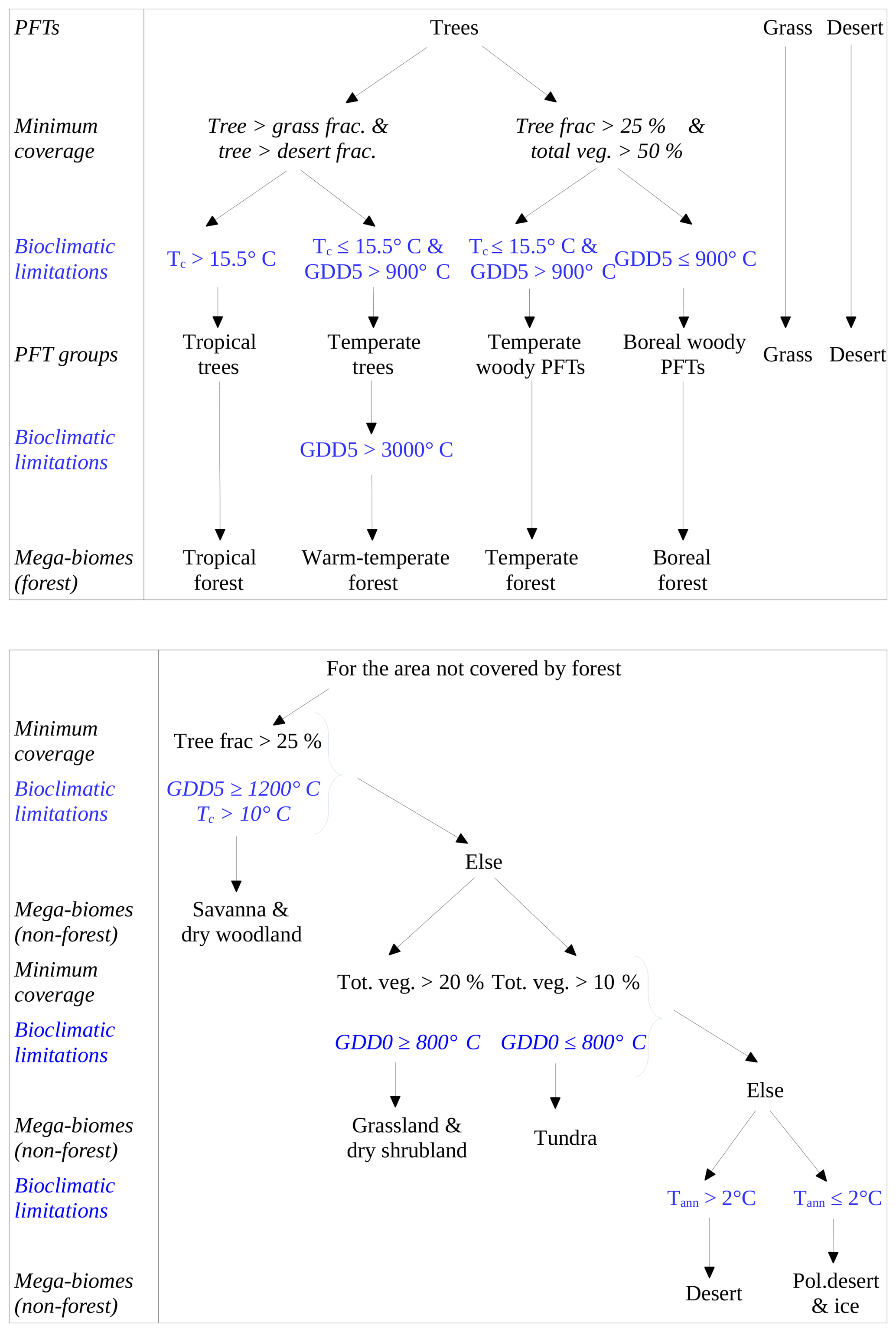
Figure A1The PFT-biomisation procedure using the example of the VECODE model (included in CLIMBER-2), which has the fewest PFTs. Shown are all decisions using assumptions on minimum coverage of the PFTs and bioclimatic limitations, i.e. growing degree days on the basis of 0 and 5∘ (GDD0, GDD5), mean temperature of the coldest month (Tc) and annual mean 2 m temperature. Please note that this chart looks different for every other model.
The MPI-ESM-P (Giorgetta et al., 2013) simulations have been performed at the Max Planck Institute for Meteorology and include the land model JSBACH with dynamic vegetation module (cf. Reick et al., 2013). In the pre-industrial control simulation, vegetation pattern and land use were prescribed. For the palaeo-simulations, we use the simulations with interactive vegetation. The spatial resolution for the atmosphere and land is T63 (i.e. approximately 1.875∘ on a Gaussian grid). These simulations are referred to as MPI-ESM-T63 in the following. In a similar model setup, additional PMIP3-like experiments have been undertaken for PI and LGM by Klockmann et al. (2016) in a coarser spatial resolution (T31, i.e. approximately 3.75∘ on a Gaussian grid, MPI-ESM-T31).
IPSL-CM5A-LR (Dufresne et al., 2013) is the low-resolution CMIP5 model version of the Institute Pierre Simon Laplace and contains the terrestrial biosphere model ORCHIDEE (Krinner et al., 2005) that is run offline, forced with climate input. In the PMIP3 simulations, vegetation and land use were prescribed. For better comparison with the gridded reference dataset (see next section), the climate and PFT fields have been interpolated bilinearly to a Gaussian T31 grid. Using the simulated LGM climate of the PMIP3 simulation, Zhu et al. (2018) performed additional experiments for LGM with ORCHIDEE-MICT (Guimberteau et al., 2018), a model version with an improved vegetation dynamic in the high northern latitudes (Zhu et al., 2015). The corresponding PI control simulation has been forced by CRUNCEP v.5.3.2 data, which are a combination of observations (CRU data) and reanalysis data (NCEP). The simulations have been interpolated to a Gaussian T63 grid.
HadGEM2-ESM (Collins et al., 2011) is the Earth system model of the Met Office Hadley Centre and includes the vegetation model TRIFFID (Cox, 2001). In all simulations used here, the model ran with interactive vegetation. The PI simulation (piControl) included land-use types. The simulations have been remapped to a Gaussian T63 grid.
The dynamic vegetation LPJ model (Sitch et al., 2003) is usually used for offline simulations, forced by climate simulations or observations. The simulations used here have been conducted in a similar model setup to that described in Kleinen et al. (2010) but has been redone on a new computer (Thomas Kleinen, personal communication, 2017), which may lead to very small deviations from the original runs. The PI simulation has been forced by observational datasets (CRU TS3.1; Harris et al., 2014), the 6 ka simulation by output from the CLIMBER-2 model. Both simulations have been interpolated to a Gaussian T63 grid and are referred to as CLIM-LPJ in the following text.
MIROC-ESM (Watanabe et al., 2011) is the Earth system model of the Japan Agency for Marine-Earth Science and Technology, Atmosphere and Ocean Research Institute (University of Tokyo) and the National Institute for Environmental Studies. It includes the SEIB dynamic vegetation model (Sato et al., 2007). SEIB deviates from the other DGVMs in this study as it does not use the tiling approach of calculating PFT fractional coverage for each grid cell. It is a so-called gap model, simulating the interactions among individual trees that compete for light and space in arising gaps (e.g. due to disturbances) within a spatially explicit virtual forest. The model was built for capturing the vegetation dynamics on a local scale. The application of the model for larger (e.g. global) scales is possible, but global simulations partly disagreed with observations (Sato et al., 2007). The PFT distribution used in this study has been calculated in the post-processing for CMIP5 via the relative net primary productivity of the vegetation categories; it was not explicitly calculated by the model, which may lead to additional biases in the vegetation distribution. The simulation for PI (piControl) includes land use. These simulations have been remapped to a Gaussian T31 grid.
CLIMBER-2 (Petoukhov et al., 2000) is an Earth system model of intermediate complexity and contains the vegetation module VECODE (Brovkin et al., 1997). The LGM and PI simulations have been specifically undertaken for this study (Thomas Kleinen, personal communication, 2017) and are referred to as CLIMBER in the following. The CLIMBER output has not been interpolated as the simulation ran with a too-coarse resolution of 10∘ latitude × 51∘ longitude. To compare with the data and the other models, the CLIMBER output was regridded to grid without interpolation.
The dynamic global vegetation model CLM-DGVM as part of the Community Earth System Model (Hurrell et al., 2013) is currently under redevelopment. No appropriate simulations could be provided.
Most biomes used in RF99 could directly be assigned to the mega-biome types used in this study (Table C1). RF99 additionally includes the biome “evergreen/deciduous mixed forest/woodland”. Here, this biome is assigned to the mega-biomes “temperate forest” in warm regions and “boreal forest” in colder regions via the modern growing degree day distribution (GDD5 ≥ 900 ∘C for warm regions, GDD5 < 900 ∘C for cold regions; cf. Table 2), derived from observations (University of East Anglia Climatic Research Unit Time Series 3.1, University of East Anglia, 2008). Likewise, the savanna biome had to be split up, as RF99 includes temperate savanna which is explicitly excluded in the definition of the savanna mega-biome used in this study. The threshold for warm savanna is a mean temperature of the coldest month exceeding 10 ∘C (limit for existence of C4 grass in JSBACH). To compare RF99 with the different model simulations, RF99 had to be remapped to the model grids. We decided to use the spatial resolutions T31 and T63, and also prepared a map for the downscaled CLIMBER output ( grid). Within each of these model grid cells, the dominant mega-biome type in the 5 min resolved RF99 data was taken for covering the RF99 grid box in T31 or T63 or in the 10∘ grid. In more detail, each grid box on a T31 Gaussian grid contains 45 × 45 grid cells of the 5 min resolved RF99 data. Within these 45 × 45 grid boxes, the fractional coverage of all mega-biomes is calculated and the biome with the highest fraction is chosen for covering the T31 grid box. For T63, arithmetically 22.5 × 22.5 grid cells form one T63 grid cell. Here, we take 23 × 23 RF99 grid boxes with one grid-box overlap to equally distribute the 5 min grid cells to the T63 grid. We are aware of the fact that the latitudes in the Gaussian grids are actually not equidistant, so that the remapped RF99 biome distributions are slightly stretched towards the poles, but this effect is marginal and is not expected to shift the main biome belts. To compare the equal number of grid cells, the reference data are cut by the land–sea masks used in the individual simulations to only include grid cells that are on land in both datasets.
Table C1Biome assignment of biome classes used in Ramankutty and Foley (1999) to the mega-biomes used in this study.
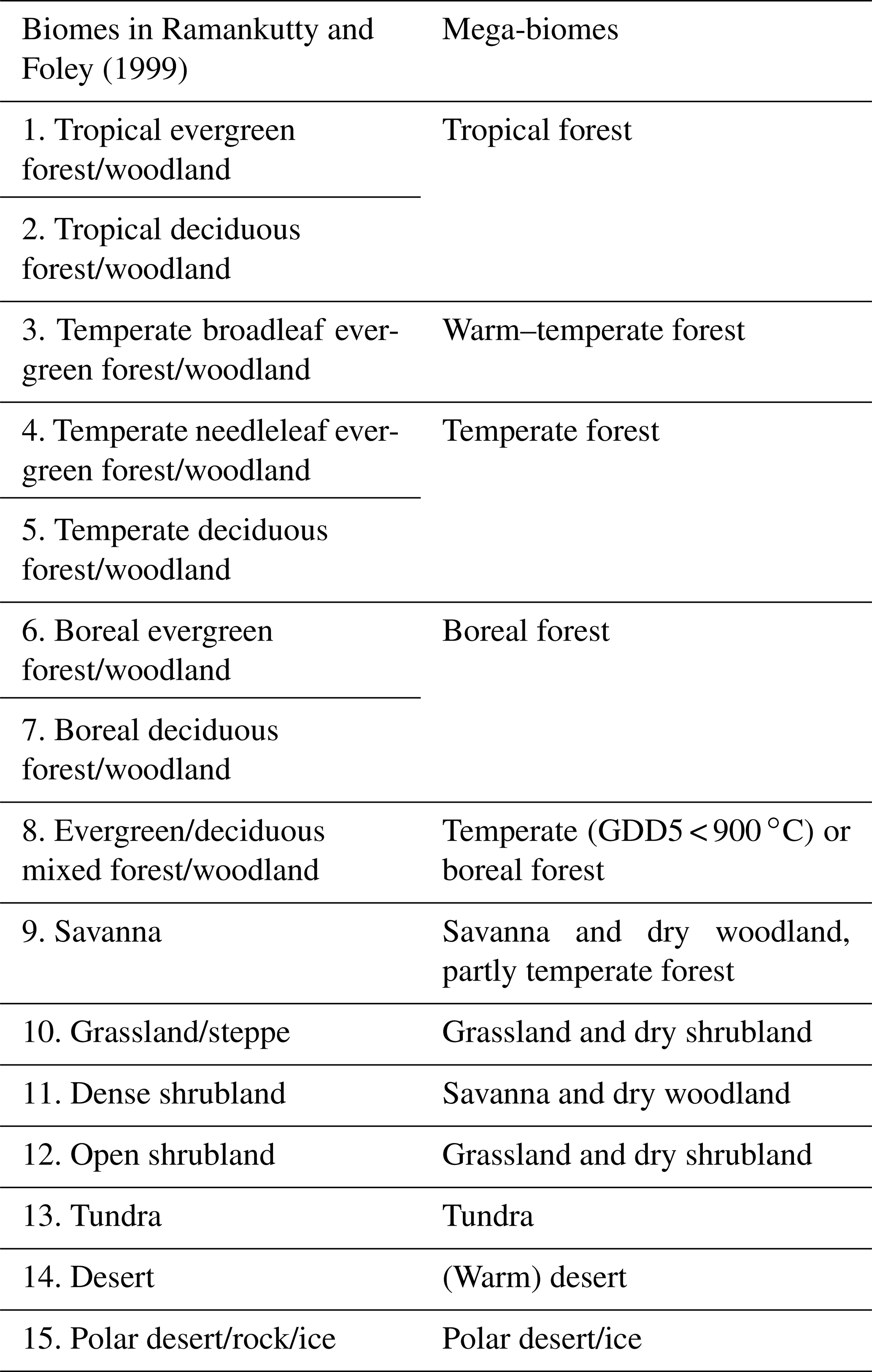
Table D1Modern (PI) fraction of the biome “tropical forest” in South America, given in percent of land area in the region of 57∘ S–13∘ N, 33–81∘ W. Listed are the reference forest fraction based on RF99, which changes due to the interpolation to the different model grids, the forest fraction based on the PFT biomisation and that based on the classical approach using BIOME1 forced with the simulated climate fields.
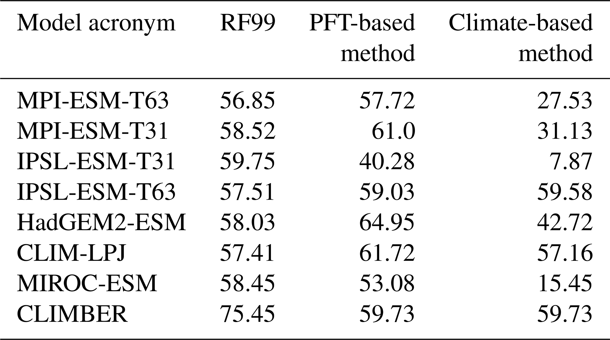
Prentice et al. (2011) introduced a biomisation method (further referred to as the FPC method) that is fundamentally different from the method presented in this study. The assignment to the different biomes is controlled by the foliage projective cover, the vegetation height and the PFT composition. Climatic limitations in the form of growing degree days are only used to distinguish the tundra biomes.
Unfortunately, the foliage projective cover and the vegetation height are not included in the standard output of the vegetation models and are therefore not available for the simulations used here.
To compare both methods, we therefore only use the simulations performed within IPSL-ESM-T63, which has been biomised by Zhu et al. (2018) following the approach of Prentice et al. (2011). The biome output has been grouped into mega-biomes and remapped to a T63 grid in the same way as the RF99 reference data were prepared.
Beside the savanna regions, the derived biome map resembles the map resulting from the PFT-based method (Fig. E1). Prentice et al. distinguish between temperate parkland, sclerophyll woodland and boreal parkland that all have been assigned to the mega-biome savanna, but savanna is only defined as tropical savanna in our method. This complicates the comparison of the biome maps and leads to strong differences in the savanna distribution between both methods and between the biomisation using the FPC method and RF99, although we leave the temperate savanna in RF99 for better comparison.
Since boreal parkland is not included in RF99, the PFT method introduced here yields better results for boreal forest and savanna than the FPC method. Additionally, the warm–temperate forest is more appropriately reproduced. In contrast, temperate forest and grassland are better represented using the FPC method. All other biomes are equally well simulated for the PI time slice.
Table E1Metrics quantifying the agreement of the biomisations for IPSL-ESM-T63 based on the FPC method (Prentice et al., 2011) or the PFT-based method introduced in this study with the modern potential biome distribution according to Ramakutty and Foley (1999, RF99) or pollen-based biome reconstructions (BIOME6000 database) for the pre-industrial (PI) and the Last Glacial Maximum (LGM) time slices. Listed are the relative fractional skill score (FSS), the kappa value (κ) and the best neighbour score (BNS).
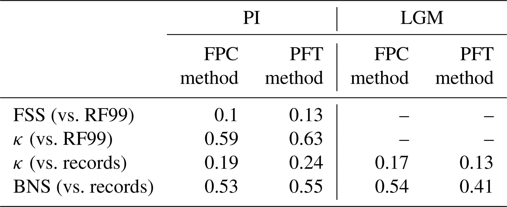
The FSS metric (Table E1) indicates that the PFT-based method (0.13) agrees in total slightly better with the reference than the other approach (0.10). Overall, the biomisation using the FPC method reaches a κ of 0.59 (vs. 0.63 for the PFT-based method) compared to RF99 and 0.19 (vs. 0.24) compared to the Biome6000 pollen data. BNS is 0.53 for the FPC method and 0.55 for the PFT method.
The LGM biome distribution can be captured slightly better using the FPC method (k=0.17 vs. 0.13 and BNS = 0.54 vs. 0.41). Particularly the tropical forest, desert and savanna biomes agree better with the biome reconstructions than those for the PFT-based method, but at least for the latter biomes, the record density is very low, which may distort the results.
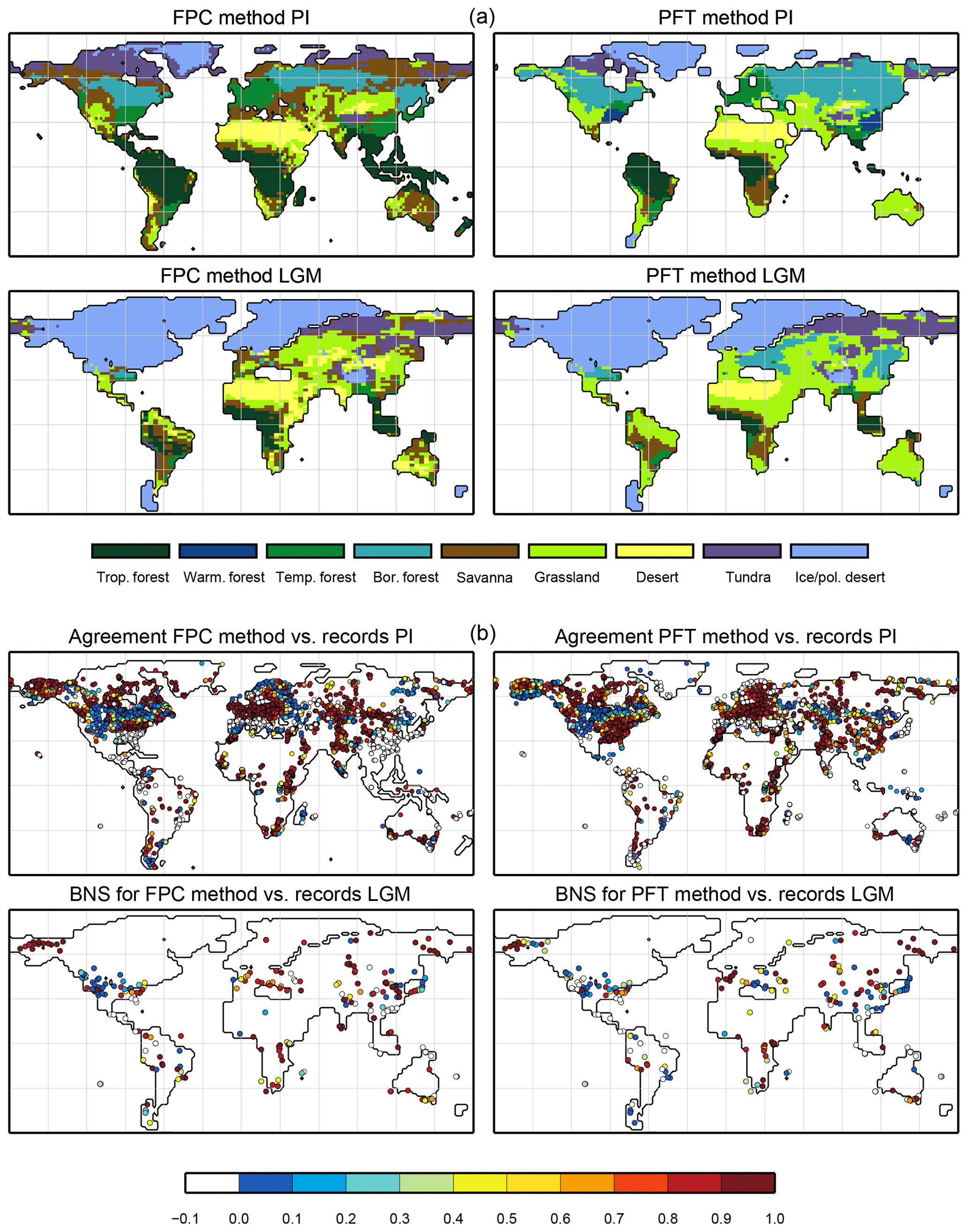
Figure E1Comparison between the biomisation method by Prentice et al. (2011, referred to as the FPC method) and the method introduced in this study (PFT-based) based on the IPSL-ESM-T63 model. Shown are the biome distributions for the pre-industrial (PI) and Last Glacial Maximum (LGM) time slices (a) and the BNS for all available sites showing the agreement of the reconstructed biomes (according to the BIOME6000 database) and the simulated biome distributions in the neighbourhood of the sites (b), ranging from 0 (no grid cell in the surrounding shows the same biome as reconstructed) to 1 (the grid cell locating the site and the record at the site indicate the same biome). Please notice that the FPC method distinguishes temperate parkland, sclerophyll woodland and boreal parkland, which all have been assigned to the mega-biome savanna, but savanna is only defined as tropical savanna in the PFT method.
All authors contributed to the development of the method. AD performed the biomisations and prepared the paper. All authors discussed the analysis and the paper.
The authors declare that they have no conflict of interest.
This work contributes to the project PalMod, funded by the German Federal Ministry of Education and Research (BMBF), Research for Sustainability initiative (FONA, https://www.fona.de, last access: 8 February 2019). Anne Dallmeyer was financed by PalMod. We thank Julian Koch (GEUS) for fruitful discussion on metrics, Jian Ni (ZJNU) and Ulrike Herzschuh (AWI) for the help on the pollen-based biomisation and Thomas Kleinen (MPI-M) for performing the CLIMBER and CLIM-LPJ simulations and his helpful comments on an earlier version of this paper. Many thanks go to Reiner Schnur (MPI-M) for the technical help. We furthermore would like to acknowledge Dan Zhu (IPSL) for providing the IPSL-ESM-T63 simulations and the biome data derived by the FPC-biomisation method. We would like to thank the editor, Denis-Didier Rousseau, for kindly handling this paper and the three anonymous referees for their constructive comments which helped to significantly improve the manuscript.
We acknowledge the World Climate Research Programme's Working Group on
Coupled Modelling, which is responsible for CMIP, and we thank the climate
modelling groups (listed in Sect. 2.2 of this paper) for producing and
making available their model output. For CMIP, the US Department of
Energy's Program for Climate Model Diagnosis and Intercomparison provides
coordinating support and led the development of software infrastructure in
partnership with the Global Organization for Earth System Science Portals.
The article processing charges for this open-access
publication were covered by the Max Planck Society.
Edited by: Denis-Didier Rousseau
Reviewed by: Jed Kaplan and two anonymous referees
Bigelow, N. H., Brubaker, L. B., Edwards, M. E., Harrison, S. P., Prentice, I. C., Anderson, P. M., Andreev, A. A., Bartlein, P. J., Christensen, T. R., Cramer, W., Kaplan, J. O., Lozhkin, A. V., Matveyeva, N. V., Murray, D. F., McGuire, A. D., Razzhivin, A. Y., Ritchie, J. C., Smith, B., Walker, D. A., Galjewski, K., Wolf, V., Holmquist, B., Igarashi, Y., Kremenetskii, K., Paus, A., Pisaric, M. F. J., and Volkova, V. S.: Climate change and Arctic ecosystems – I. Vegetation changes north of 50∘ N between the last glacial maximum, mid-Holocene and present, J. Geophys. Res., 108, 8170, https://doi.org/10.1029/2002JD002558, 2003.
Braconnot, P., Harrison, S. P., Otto-Bliesner, B., Abe-Ouchi, A., Jungclaus, J., and Peterschmitt, J. Y.: The Paleoclimate Modeling Intercomparison Project contribution to CMIP5, CLIVAR Exchanges No. 56, 16, 15–19, 2011.
Brovkin, V., Ganopolski, A., and Svirezhev, Y.: A continuous climate-vegetation classification for use in climate-biosphere studies, Ecol. Model., 101, 251–261, 1997.
Calvo, M. and Prentice, I. C.: Effects of fire and CO2 on biogeography and primary production in glacial and modern climates, New Phytol., 208, 987–994, https://doi.org/10.1111/nph.13485, 2015.
Chen, Y., Ni, J., and Herzschuh, U.: Quantifying modern biomes based on surface pollen data in China, Global Planet. Change, 74, 114–131, 2010.
Cohen, J.: A coefficient of agreement for nominal scales, Educ. Psychol. Meas., 20, 37–46, 1960.
Collins, W. J., Bellouin, N., Doutriaux-Boucher, M., Gedney, N., Halloran, P., Hinton, T., Hughes, J., Jones, C. D., Joshi, M., Liddicoat, S., Martin, G., O'Connor, F., Rae, J., Senior, C., Sitch, S., Totterdell, I., Wiltshire, A., and Woodward, S.: Development and evaluation of an Earth-System model – HadGEM2, Geosci. Model Dev., 4, 1051–1075, https://doi.org/10.5194/gmd-4-1051-2011, 2011.
Cox, P. M.: Description of the TRIFFID dynamic global vegetation model, Technical note 24, Hadley Centre, Met Office, Exeter, UK, 2001.
Crucifix, M., Betts, R. A., and Hewitt, C. D.: Pre-industrial potential and Last Glacial Maximum global vegetation simulated with a coupled climate-biosphere model: diagnosis of bioclimatic relationships, Global Planet. Change, 45, 295–312, 2005.
Dallmeyer, A., Claussen, M., Ni, J., Cao, X., Wang, Y., Fischer, N., Pfeiffer, M., Jin, L., Khon, V., Wagner, S., Haberkorn, K., and Herzschuh, U.: Biome changes in Asia since the mid-Holocene – an analysis of different transient Earth system model simulations, Clim. Past, 13, 107–134, https://doi.org/10.5194/cp-13-107-2017, 2017.
Diffenbaugh, N. S., Sloan, L. C., Snyder, M. A., Bell, J. L., Kaplan, J., Shafer, S. L., and Bartlein, P. J.: Vegetation sensitivity to global anthropogenic carbon dioxide emissions in a topographically complex region, Global Biogeochem. Cy., 17, 1067, https://doi.org/10.1029/2002GB001974, 2003.
Dufresne, J.-L., Foujols, M.-A., Denvil, S., Caubel, A., Marti, O., Aumont, O., Balkanski, Y., Bekki, S., Bellenger, H., Benshila, R., Bony, S., Bopp, L., Braconnot, P., Brockmann, P., Cadule, P., Cheruy, F., Codron, F., Cozic, A., Cugnet, D., de Noblet, N., Duvel, J.-P., Ethé, C., Fairhead, L., Fichefet, T., Flavoni, S., Friedlingstein, P., Grandpeix, J.-Y., Guez, L., Guilyardi, E., Hauglustaine, D., Hourdin, F., Idelkadi, A., Ghattas, J., Joussaume, S., Kageyama, M., Krinner, G., Labetoulle, S., Lahellec, A., Lefebvre, M.-P., Lefevre, F., Levy, C., Li, Z. X., Lloyd, J., Lott, F., Madec, G., Mancip, M., Marchand, M., Masson, S., Meurdesoif, Y., Mignot, J., Musat, I., Parouty, S., Polcher, J., Rio, C., Schulz, M., Swingedouw, D., Szopa, S., Talandier, C., Terray, P., Viovy, N., and Vuichard, N.: Climate change projections using the IPSL-CM5 Earth System Model: from CMIP3 to CMIP5, Clim. Dynam., 40, 2123, https://doi.org/10.1007/s00382-012-1636-1, 2013.
Foody, G. M.: Status of land cover classification accuracy assessment, Remote Sens. Environ., 80, 185–201, 2002.
Franco, A. C., Rossatto, D. R., de Carvalho Ramos Silva, L., and da Silva Ferreira, C.: Cerrado vegetation and global change: the role of functional types, resource availability and disturbance in regulating plant community responses to rising CO2 levels and climate warming, Theor. Exp. Plant Physiol., 26, 19–38, https://doi.org/10.1007/s40626-014-0002-6, 2014.
Gilleland, E., Ahijevych, D., Brown, B. G., Casati, B., and Ebert, E. E.: Intercomparison of spatial forecast verification methods, Weather Forecast., 24, 1416–1430, https://doi.org/10.1175/2009WAF2222269.1, 2009.
Giorgetta, M. A., Jungclaus, J., Reick, C. H., Legutke, S., Bader, J., Böttinger, M., Brovkin, V., Crueger, T., Esch, M., Fieg, K., Glushak, K., Gayler, V., Haak, H., Hollweg, H.-D., Ilyina, T., Kinne, S., Kornblueh, L., Matei, D., Mauritsen, T., Mikolajewicz, U., Mueller, W., Notz, D., Pithan, F., Raddatz, T., Rast, S., Redler, R., Roeckner, E., Schmidt, H., Schnur, R., Segschneider, J., Six, K. D., Stockhause, M., Timmreck, C., Wegner, J., Widmann, H., Wieners, K.-H., Claussen, M., Marotzke, J., and Stevens, B.: Climate and carbon cycle changes from 1850 to 2100 in MPI-ESM simulations for the Coupled Model Intercomparison Project phase 5, J. Adv. Model. Earth Syst., 5, 572–597, https://doi.org/10.1002/jame.20038, 2013.
Guimberteau, M., Zhu, D., Maignan, F., Huang, Y., Yue, C., Dantec-Nédélec, S., Ottlé, C., Jornet-Puig, A., Bastos, A., Laurent, P., Goll, D., Bowring, S., Chang, J., Guenet, B., Tifafi, M., Peng, S., Krinner, G., Ducharne, A., Wang, F., Wang, T., Wang, X., Wang, Y., Yin, Z., Lauerwald, R., Joetzjer, E., Qiu, C., Kim, H., and Ciais, P.: ORCHIDEE-MICT (v8.4.1), a land surface model for the high latitudes: model description and validation, Geosci. Model Dev., 11, 121–163, https://doi.org/10.5194/gmd-11-121-2018, 2018.
Hagen, A.: Fuzzy set approach to assessing similarity of categorical maps, Int. J. Geogr. Inf. Sci., 17, 235–249, 2003.
Hagen, A.: An improved Fuzzy Kappa statistic that accounts for spatial autocorrelation, Int. J. Geogr. Inform. Sci., 23, 61–73, 2009.
Handiani, D., Paul, A., and Dupont, L.: Tropical climate and vegetation changes during Heinrich Event 1: a model-data comparison, Clim. Past, 8, 37–57, https://doi.org/10.5194/cp-8-37-2012, 2012.
Handiani, D., Paul, A., Prange, M., Merkel, U., Dupont, L., and Zhang, X.: Tropical vegetation response to Heinrich Event 1 as simulated with the UVic ESCM and CCSM3, Clim. Past, 9, 1683–1696, https://doi.org/10.5194/cp-9-1683-2013, 2013.
Harris, I., Jones, P. D., Osborn, T. J., and Lister, D. H.: Updated high-resolution grids of monthly climatic observations – the CRU TS3.10 Dataset, Int. J. Climatol., 34, 623–642, https://doi.org/10.1002/joc.3711, 2014.
Harrison, S.: BIOME 6000 DB classified plotfile version 1, University of Reading, Dataset, https://doi.org/10.17864/1947.99 , 2017.
Harrison, S., Bartlein, P. J., and Prentice, C. I.: What have we learnt from paleoclimate simulations?, J. Quaternary Sci., 31, 363–385, 2016.
Harrison, S. P. and Prentice, I. C.: Climate and CO2 controls on global vegetation distribution at the last glacial maximum: analysis based on palaeovegetation data, biome modelling and palaeo climate simulations, Glob. Change Biol., 9, 983–1004, 2003.
Harrison, S. P., Prentice, I. C., Barboni, D., Kohfeld, K., Ni, J., and Sutra, J.-P.: Ecophysiological and bioclimatic foundations for a global plant functional classification, J. Veg. Sci., 21, 300–317, https://doi.org/10.1111/j.1654-1103.2009.01144.x, 2010.
Haxeltine, A. and Prentice, C. I.: BIOME3: An equilibrium terrestrial biosphere model based on ecophysiological constraints, resource availability, and competition among plant functional types, Global Biogeochem. Cy., 10, 693–709, 1996.
Hurrell, J. W., Holland, M. M., Gent, P. R., Ghan, S., Kay, J. E., Kushner, P. J., Lamarque, J., Large, W. G., Lawrence, D., Lindsay, K., Lipscomb, W. H., Long, M. C., Mahowald, N., Marsh, D. R., Neale, R. B., Rasch, P., Vavrus, S., Vertenstein, M., Bader, D., Collins, W. D., Hack, J. J., Kiehl, J., and Marshall, S.: The Community Earth System Model: A Framework for Collaborative Research, B. Am. Meteorol. Soc., 94, 1339–1360, https://doi.org/10.1175/BAMS-D-12-00121.1, 2013
Jacobson Jr., G. L. and Bradshaw, R. H. W.: The selection of sites for paleovegetational studies, Quateranry Res., 16, 80–96, 1981.
Jolly, D., Harrison, S. P., Damnati B., and Bonnefille, R.: Simulated climate and biomes of Africa during the Late Quaternary: comparison with pollen and lake status data, Quaternary Sci. Rev., 17, 629–657, 1998.
Jones, H. T., Mayle, F. E., Pennington, R. T., and Killeen, T. J.: Characterisation of Bolivian savanna ecosystems by their modern pollen rain and implications for fossil pollen records, Rev. Palaeobot. Palyno., 164, 223–237, https://doi.org/10.1016/j.revpalbo.2011.01.001, 2011.
Kageyama, M., Braconnot, P., Bopp, L., Mariotti, V., Roy, T., Woillez, M.-N., Caubel, A., Foujols, M.-A., Guilyardi, E., Khodri, M., Lloyd, J., Lombard, F., and Marti, O.: Mid-Holocene and last glacial maximum climate simulations with the IPSL model: part II: model-data comparisons, Clim. Dynam., 40, 2469, https://doi.org/10.1007/s00382-012-1499-5, 2013.
Kaplan, J. O., Bigelow, N. H., Prentice, I. C., Harrison, S. P., Bartlein, P. J., Christensen, T. R., Cramer, W., Matveyeve, N. V., McGuire, A. D., Murray, D. F., Razzhivin, V. Y., Smith, B., Walker, D. A., Anderson, P. M., Andreev, A. A., Brubaker, L. B., Edwards, M. E., and Lozhkin, A. V.: Climate change and arctic ecosystems: 2. Modeling, paleodata-model comparisons, and future projections, J. Geophys. Res., 108, 8171, https://doi.org/10.1029/2002JD002559, 2003.
Kleinen, T., Brovkin, V., von Bloh, W., Archer, D., and Munhoven, G.: Holocene carbon cycle dynamics, Geophys. Res. Lett., 37, L2705, https://doi.org/10.1029/2009GL041391, 2010.
Klockmann, M., Mikolajewicz, U., and Marotzke, J.: The effect of greenhouse gas concentrations and ice sheets on the glacial AMOC in a coupled climate model, Clim. Past, 12, 1829–1846, https://doi.org/10.5194/cp-12-1829-2016, 2016.
Koch, J., Mendiguren, G., Mariethoz, G., and Stisen, S.: Spatial sensitivity analysis of simulated land-surface patterns in a catchment model using a set of innovative spatial performance metrics, J. Hydrometeorol., 18, 1121–1142, https://doi.org/10.1175/JHM-D-16-0148.1, 2017.
Krinner, G., Viovy, N., de Noblet-Ducoudre, N., Ogee, J., Polcher, J., Friedlingstein, P., Ciais, P., Sitch, S., and Prentice, I. C.: A dynamic global vegetation model for studies of the coupled atmosphere-biosphere system, Global Biogeochem. Cy., 19, Gb1015, https://doi.org/10.1029/2003gb002199, 2005.
Landis, J. R. and Koch, G. G.: Application of hierarchical Kappa-type statistics in assessment of majority agreement among multiple observers, Biometrics, 33, 363–374, 1977.
Lehmann, C. E. R., Archibald, S. A., Hoffmann, W. A., and Bond, W. J.: Deciphering the distribution of the savanna biome, New Phytol., 191, 197–209, https://doi.org/10.1111/j.1469-8137.2011.03689.x, 2011.
Loranty, M. M., Berner, L. T., Goetz, S. J., Jin, Y., and Randerson, J. T.: Vegetation controls on northern high latitude snow-albedo feedback: observations and CMIP5 model predictions, Glob. Change Biol., 20, 594–606, https://doi.org/10.1111/gcb.12391, 2013.
Mittermaier, M., Roberts, N., and Thompson, S. A.: A long-term assessment of precipitation forecast skill using the fractions skill score, Meteor. Appl., 20, 176–186, https://doi.org/10.1002/met.296, 2013.
Monserud, R. A. and Leemans, R.: Comparing global vegetation maps with the Kappa statistic, Ecol. Model., 62, 275–293, 1992
Ni, J., Yu, G., Harrison, S. P., and Prentice, I. C.: Palaeovegetation in China during the late Quaternary: biome reconstructions based on a global scheme of plant functional types, Palaeogeogr. Palaeocl., 289, 44–61, 2010.
Petoukhov, V., Ganopolski, A., Brovkin, V., Claussen, M., Eliseev, A., Kubatzki, C., and Rahmstorf, S.: CLIMBER-2: A climate system model of intermediate complexity, Clim. Dynam., 16, 1–17, 2000.
Prentice, I. C., Cramer, W., Harrison, S. P., Leemans, R., Monserud, R. A., and Solomon, A. M.: A global biome model based on plant physiology and dominance, soil properties and climate, J. Biogeogr., 19, 117–134, 1992.
Prentice, I. C., Guiot, J., Huntley, B., Jolly, D., and Cheddadi, R.: Reconstructing biomes from palaeoecological data: a general method and its application to European pollen data at 0 and 6 ka, Clim. Dynam., 12, 185–194, 1996.
Prentice, I. C. and Webb III, T.: BIOME 6000: reconstructing global mid-Holocene vegetation patterns from palaeoecological records, J. Biogeogr., 25, 997–1005, 1998.
Prentice, I. C., Jolly, D., and BIOME 6000 participants: Mid-Holocene and glacial maximum vegetation geography of the northern continents and Africa, J. Biogeogr., 27, 507–519, 2000.
Prentice, I. C, Bondeau, A., Cramer, W., Harrison, S. P., Hickler, T., Lucht, W., Sitch, S., Smith, B., and Sykes, M.: Dynamic Global Vegetation Modeling: quantifying terrestrial ecosystem responses to large-scale environmental change, in: Terrestrial ecosystems in a changing world, edited by: Canadell, J. G., Pataki, D. E., and Pitelka, L. F., Berlin, Germany, Springer, 175–192, 2007.
Prentice, I. C., Harrison, S. P., and Bartlein, P. J.: Global vegetation and terrestrial carbon cycle changes after the last ice age, New Phytol., 189, 988–998, 2011.
Ramankutty, N. and Foley, J. A.: Estimating historical changes in global land cover: croplands from 1700 to 1992, Global Biogeochem. Cy., 13, 997–1027, 1999.
Ratnam, J., Bond, W. J., Fensham, R. J., Hoffmann, W. A., Archibald, S., Lehmann, C. E. R., Anderson, M. T., Higgins, S. I., and Sankaran, M.: When is a “forest” a savanna, and why does it matter?, Glob. Ecol. Biogeogr., 20, 653–660, https://doi.org/10.1111/j.1466-8238.2010.00634.x, 2011.
Reick, C. H., Raddatz, T., Brovkin, V., and Gayler, V.: Representation of natural and anthropogenic land cover change in MPI-ESM, J. Adv. Model. Earth Syst., 5, 459–482, 2013.
Roberts, N. M. and Lean, H. W.: Scale-selective verification of rainfall accumulations from high-resolution forecasts of convective events, Mon. Wether Rev., 136, 78–97, https://doi.org/10.1175/2007MWR2123.1, 2008.
Roche, D. M., Dokken, T. M., Goosse, H., Renssen, H., and Weber, S. L.: Climate of the Last Glacial Maximum: sensitivity studies and model-data comparison with the LOVECLIM coupled model, Clim. Past, 3, 205–224, https://doi.org/10.5194/cp-3-205-2007, 2007.
Sato, H., Itoh, A., and Kohyama, T.: SEIB-DGVM: A New Dynamic Global Vegetation Model using a Spatially Explicit Individual-Based Approach, Ecol. Model., 200, 279–307, https://doi.org/10.1016/j.ecolmodel.2006.09.006, 2007.
Scholes, D. and Hall, R.: The carbon budget of tropical savannas; woodlands and grasslands, in: Global change: effects on; coniferous forests and grassland, edited by: Breymeyer, A. I., Hall, I. D., Melillo, J. M., and Agren, G. I., Wiley, New York, 69–100, 1996.
Schurgers, G., Mikolajewicz, U., Groeger, M., Maier-Reimer, E.,Vizcaıno, M., and Winguth, A.: Dynamics of the terrestrial biosphere, climate and atmospheric CO2 concentration during interglacials: a comparison between Eemian and Holocene, Clim. Past, 2, 205–220, https://doi.org/10.5194/cp-2-205-2006, 2006.
Sitch, S., Smith, B., Prentice, I. C., Arneth, A., Bondeau, A., Cramer, W., Kaplan, J. O., Levis, S., Lucht, W., Sykes, M. T., Thonicke, K., and Venevsky, S.: Evaluation of ecosystem dynamics, plant geography and terrestrial carbon cycling in the LPJ dynamic global vegetation model, Glob. Change Biol., 9, 161–185, 2003.
Sykes, M. T., Prentice, I. C., and Laarif, F.: Quantifying the impact of global climate change on potential natural vegetation, Climatic Change, 41, 37–52, https://doi.org/10.1023/A:1005435831549, 1999.
Tang, G., Shafer, S. L., Bartlein, P., and Holman, J.: Effects of experimental protocol on global vegetation model accuracy: a comparison of simulated and observed vegetation patterns for Asia, Ecol. Model., 220, 1481–1491, 2009.
Taylor, K. E., Stouffer, R. J., and Meehl, G. A.: An Overview of CMIP5 and the experiment design, B. Am. Meteorol. Soc., 93, 485–498, https://doi.org/10.1175/BAMS-D-11-00094.1, 2012.
Tian, F., Cao, X., Dallmeyer, A., Lohmann, G., Zhang, X., Ni, J., Andreev, A., Anderson, P., Lozhkin, A., Bezrukova, E., Rudaya, N., Xu, Q., and Herzschuh, U.: Biome changes and their inferred climatic drivers in northern and eastern continental Asia at selected times since 40 cal ka bp, Veg. Hist. Archaeobot., 27, 365–379, https://doi.org/10.1007/s00334-017-0653-8, 2018.
Torello-Raventos, M., Feldpausch, T. R., Veenendaal, E., Schrodt, F., Saiz, G., Domingues, T. F., Djagbletey, G., Ford, A., Kemp, J., Marimon, B. S., Hur Marimon Junior, B., Lenza, E., Ratter, J. A., Maracahipes, L., Sasaki, D., Sonké, B., Zapfack, L., Taedoumg, H., Villarroel, D., Schwarz, M., Quesada, C. A., Yoko Ishida, F., Nardoto, G. B., Affum-Baffoe, K., Arroyo, L., M. J. S. Bowman, D., Compaore, H., Davies, K., Diallo, A., Fyllas, N. M., Gilpin, M., Hien, F., Johnson, M., Killeen, T. J., Metcalfe, D., Miranda, H. S., Steininger, M., Thomson, J., Sykora, K., Mougin, E., Hiernaux, P., Bird, M. I., Grace, J., Lewis, S. L., Phillips, O. L., and Lloyd, J.: On the delineation of tropical vegetation types with an emphasis on forest/savanna transitions, Plant Ecol. Divers., 6, 101–137, https://doi.org/10.1080/17550874.2012.762812, 2013.
University of East Anglia Climatic Research Unit (Jones, P. D. and Harris, I. C.): Climatic Research Unit (CRU) time-series datasets of variations in climate with variations in other phenomena, NCAS British Atmospheric Data Centre, available at: http://catalogue.ceda.ac.uk/uuid/3f8944800cc48e1cbc29a5ee12d8542d (last access: 1 November 2011), 2008.
University of East Anglia Climatic Research Unit (Harris, I. C. and Jones, P. D.): CRU TS4.00: Climatic Research Unit (CRU) Time-Series (TS) version 4.00 of high-resolution gridded data of month-by-month variation in climate (January 1901–December 2015), Centre for Environmental Data Analysis, https://doi.org/10.5285/edf8febfdaad48abb2cbaf7d7e846a86, 2017.
Watanabe, S., Hajima, T., Sudo, K., Nagashima, T., Takemura, T., Okajima, H., Nozawa, T., Kawase, H., Abe, M., Yokohata, T., Ise, T., Sato, H., Kato, E., Takata, K., Emori, S., and Kawamiya, M.: MIROC-ESM 2010: model description and basic results of CMIP5-20c3m experiments, Geosci. Model Dev., 4, 845–872, https://doi.org/10.5194/gmd-4-845-2011, 2011
Wohlfahrt, J., Harrison, S. P., Braconnot, P., Hewitt, C. D., Kitoh, A., Mikolajewicz, U., Otto-Bliesner, B. L., and Weaver, S. L.: Evaluation of coupled ocean-atmosphere simulations of the mid-Holocene using palaeovegetation data from the northern hemisphere extratropics, Clim. Dynam., 31, 871, https://doi.org/10.1007/s00382-008-0415-5, 2008.
Wolff, J. K., Harrold, M., Fowler, T., Gotway, J. H., Nance, L., and Brown, B. G.: Beyond the basics: Evaluating model-based precipitation forecasts using traditional, spatial, and object-based methods, Weather Forecast., 29, 1451–1472, 2014.
Zhu, D.: Modeling terrestrial carbon cycle during the Last Glacial Maximum, Thèse de doctorat Météorologie, océanographie, physique de l'environnement Paris Saclay 2016, 2016SACLV077, available at: http://www.theses.fr/2016SACLV077 (last access: 8 February 2019), 2016.
Zhu, D., Peng, S. S., Ciais, P., Viovy, N., Druel, A., Kageyama, M., Krinner, G., Peylin, P., Ottlé, C., Piao, S. L., Poulter, B., Schepaschenko, D., and Shvidenko, A.: Improving the dynamics of Northern Hemisphere high-latitude vegetation in the ORCHIDEE ecosystem model, Geosci. Model Dev., 8, 2263–2283, https://doi.org/10.5194/gmd-8-2263-2015, 2015.
Zhu, D., Ciais, P., Chang, J., Krinner, G., Peng, S., Viovy, N., Peñuelas, J., and Zimov, S.: The large mean body size of mammalian herbivores explains the productivity paradox during the Last Glacial Maximum, Nat. Ecol. Evolut., 2, 640–649, 2018.
- Abstract
- Introduction
- Methods
- Results
- Discussion
- Summary and conclusion
- Code availability
- Appendix A: Biomisation of the PFT distribution using the example of VECODE (included in CLIMBER-2)
- Appendix B: Simulations
- Appendix C: Preparing the reference datasets
- Appendix D: Simulated forest in South America
- Appendix E: Comparison of the biomisation method with the approach of Prentice et al. (2011)
- Author contributions
- Competing interests
- Acknowledgements
- References