the Creative Commons Attribution 4.0 License.
the Creative Commons Attribution 4.0 License.
 | 17 Apr 2019
Sensitivity of a leaf gas-exchange model for estimating paleoatmospheric CO2 concentration
Kylen M. Moynihan
Melissa L. McKee
Liliana Londoño
Peter J. Franks
Leaf gas-exchange models show considerable promise as paleo-CO2 proxies. They are largely mechanistic in nature, provide well-constrained estimates even when CO2 is high, and can be applied to most subaerial, stomata-bearing fossil leaves from C3 taxa, regardless of age or taxonomy. Here we place additional observational and theoretical constraints on one of these models, the “Franks” model. In order to gauge the model's general accuracy in a way that is appropriate for fossil studies, we estimated CO2 from 40 species of extant angiosperms, conifers, and ferns based only on measurements that can be made directly from fossils (leaf δ13C and stomatal density and size) and on a limited sample size (one to three leaves per species). The mean error rate is 28 %, which is similar to or better than the accuracy of other leading paleo-CO2 proxies. We find that leaf temperature and photorespiration do not strongly affect estimated CO2, although more work is warranted on the possible influence of O2 concentration on photorespiration. Leaves from the lowermost 1–2 m of closed-canopy forests should not be used because the local air δ13C value is lower than the global well-mixed value. Such leaves are not common in the fossil record but can be identified by morphological and isotopic means.
- Article
(1775 KB) -
Supplement
(83 KB) - BibTeX
- EndNote


Leaves on terrestrial plants are well poised to record information about the concentration of atmospheric CO2. They are in direct contact with the atmosphere and have large surface-area-to-volume ratios, so the leaf internal CO2 concentration is tightly coupled to atmospheric CO2 concentration. Also, leaves are specifically built for the purpose of fixing atmospheric carbon into structural tissue and face constant selection pressure to optimize their carbon uptake relative to water loss. As a result, many components of the leaf system are sensitive to atmospheric CO2, and these components feed back on one another to reach a new equilibrium when atmospheric CO2 changes. In terms of carbon assimilation, Farquhar and Sharkey (1982) modeled this system in its simplest form as
where An is the leaf CO2 assimilation rate (µmol m−2 s−1), gc(tot) is the total operational conductance to CO2 diffusion from the atmosphere to the site of photosynthesis (mol m−2 s−1), ca is atmospheric CO2 concentration (µmol mol−1 or ppm), and ci is leaf intercellular CO2 concentration (µmol mol−1 or ppm) (see also Von Caemmerer, 2000). Rearranging Eq. (1) for atmospheric CO2 yields
Equation (2) forms the basis of two leaf gas-exchange approaches for estimating paleo-CO2 from fossils (Konrad et al., 2008, 2017; Franks et al., 2014). In the Franks model, conductance is estimated in part from measurements of stomatal size and density, ci∕ca from measurements of leaf δ13C along with reconstructions of coeval air δ13C (see also Eq. 9), and An from knowledge of living relatives and its dependency on ca (Franks et al., 2014). Following Farquhar et al. (1980), the latter is modeled as (Franks et al., 2014; Kowalczyk et al., 2018)
where Γ* is the CO2 compensation point in the absence of dark respiration (ppm), and the subscript “0” refers to conditions at a known CO2 concentration (typically present day). Equations (2) and (3) are then solved iteratively until the solution for ca converges.
These gas-exchange approaches grew out of a group of paleo-CO2 proxies based on the CO2 sensitivity of stomatal density (D) or the similar metric stomatal index (Woodward, 1987; Royer, 2001). Here, the D–ca sensitivity is calibrated in an extant species, allowing for paleo-CO2 inference from the same (or very similar) fossil species. These empirical relationships typically follow a power-law function (Wynn, 2003; Franks et al., 2014; Konrad et al., 2017):
where k and α are species-specific constants.
The related stomatal ratio proxy is simplified: D is measured in an extant species (D0, at present-day ca0) and then the ratio of D0 to D in a related fossil species is assumed to be linearly related to the ratio of paleo-ca to present-day ca0 (Chaloner and McElwain, 1997; McElwain, 1998):
Equation (5) can be rearranged to match Eq. (4) but with α fixed at 1. Thus, paleo-CO2 estimates using the stomatal ratio proxy are based on a one-point calibration and an assumption that α=1; observations do not always support this assumption (e.g., α=0.43 for Ginkgo biloba; Barclay and Wing, 2016). The scalar k was originally set at 2 for Paleozoic and Mesozoic reconstructions so that paleo-CO2 estimates during the Carboniferous matched that from long-term carbon cycle models (Chaloner and McElwain, 1997). For younger reconstructions, k is probably closer to 1 (by definition, k=1 for present-day plants). We note that the stomatal ratio proxy was originally conceived as providing qualitative information only about paleo-CO2 (McElwain and Chaloner, 1995, 1996; Chaloner and McElwain, 1997; McElwain, 1998) and has not been tested with dated herbaria materials or with CO2 manipulation experiments.
At high CO2, the D–ca sensitivity saturates in many species, leading to uncertain paleo-CO2 estimates, often with unbounded upper limits (e.g., Smith et al., 2010; Doria et al., 2011). Stomatal density does not respond to CO2 in all species (Woodward and Kelly, 1995; Royer, 2001), and because D–ca relationships can be species specific (that is, different species in the same genus with different responses; Beerling, 2005; Haworth et al., 2010), only fossil taxa that are still alive today should be used. The gas-exchange proxies partly address these limitations: (1) CO2 estimates remain well-bounded – even at high CO2 – and their precision is similar to or better than other leading paleo-CO2 proxies ( % at 95 % confidence; Franks et al., 2014) and (2) the models are mostly mechanistic; that is, they are explicitly driven by plant physiological principles, not just empirical relationships measured on living plants. (3) Because the models retain sensitivity at high CO2 and do not require that a fossil species still be alive today, much of the paleobotanical record is open for CO2 inference, regardless of age or taxonomy. (4) Because the models are based on multiple inputs linked by feedbacks, they can still perform adequately even if one or more of the inputs in a particular taxon is not sensitive to CO2, for example stomatal density (Milligan et al., 2019).
We note that the published uncertainties (precision) associated with the stomatal density proxies are probably too small because they usually only reflect uncertainty in either the calibration regression or in the measured values of fossil stomatal density, but not both; when both sources are propagated, errors often exceed ±30 % at 95 % confidence (Beerling et al., 2009). Also, error rates in estimates from extant taxa for which CO2 is known (accuracy) are usually smaller with stomatal density proxies than with gas-exchange proxies (e.g., Barclay and Wing, 2016), but this is expected because the same taxa have been calibrated in present-day (or near present-day) conditions. Because the gas-exchange proxies are largely built from physiological principles, they have less “recency” bias; that is, the gas-exchange proxies estimate present-day and paleo-CO2 with similar certainty when the same methods are used to determine the inputs.
Leaf gas-exchange proxies for paleo-CO2 are becoming popular (Konrad et al., 2008, 2017; Grein et al., 2011a, b, 2013; Erdei et al., 2012; Roth-Nebelsick et al., 2012, 2014; Franks et al., 2014; Maxbauer et al., 2014; Montañez et al., 2016; Reichgelt et al., 2016; Tesfamichael et al., 2017; Kowalczyk et al., 2018; Lei et al., 2018; Londoño et al., 2018; Richey et al., 2018; Milligan et al., 2019). However, many elements in these models remain understudied. Here we scrutinize four such elements of the Franks et al. (2014) model and ask the following: how does the model perform across a large number of phylogenetically diverse taxa? And how is the model affected by temperature, photorespiration, and proximity to the forest floor? We next describe the motivation and details of the study design (see also Table 1 for a summary).
Table 1Attributes of datasets used to test the Franks et al. (2014) model.
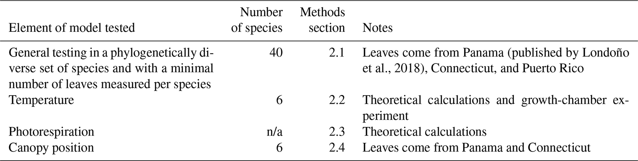
n/a: not applicable
2.1 General testing in living plants
Franks et al. (2014) tested the model on four species of field-grown trees (three gymnosperms and one angiosperm) and one conifer grown in chambers at 480 and 1270 ppm CO2. The average error rate (absolute value of estimated CO2 minus measured CO2, divided by measured CO2) was 5 %. Follow-up work with three field-grown tree species (Maxbauer et al., 2014; Kowalczyk et al., 2018), CO2 experiments on seven tropical trees species (Londoño et al., 2018), and experiments on two fern and one conifer species (Milligan et al., 2019) indicate somewhat higher error rates (Fig. 1). Combined, the average error rate is 20 % (median 13 %).

Figure 1Published CO2 estimates using the Franks model for extant plants for which the physiological inputs A0 (assimilation rate at a known CO2 concentration) and/or gc(op)∕gc(max) (ratio of operational to maximum leaf conductance to CO2) were measured directly. Horizontal lines are the correct CO2 concentrations. Uncertainties in the estimates correspond to the 16th–84th percentile range. Circles are from Londoño et al. (2018), squares from Milligan et al. (2019), large triangle from Maxbauer et al. (2014), small triangles from Kowalczyk et al. (2018), and diamonds from Franks et al. (2014).
In these studies, two of the key physiological inputs were measured directly with an infrared gas analyzer: the assimilation rate at a known CO2 concentration (A0) and/or the ratio of operational to maximum stomatal conductance to CO2 (gc(op)∕gc(max), or ζ), the latter of which is important for calculating the total leaf conductance (gc(tot)). These two inputs cannot be directly measured on fossils; thus, the error rates associated with Fig. 1 may not be representative for fossil studies. Franks et al. (2014) argue that within plant functional types growing in their natural environment, mean A0 is fairly conservative, leading to the recommended mean A0 values in Franks et al. (2014) (12 µmol m−2 s−1 for angiosperms, 10 for conifers, and 6 for ferns and ginkgos). Along similar lines, the mean ratio gc(op)/gc(max) tends to be conserved across plant functional types; Franks et al. (2014) recommend a value of 0.2, which may correspond to the most efficient set point for stomata to control conductance (Franks et al., 2012). This conservation of physiological function is one of the underlying principles in the Franks model.
Here we test this assumption by estimating CO2 from 40 phylogenetically diverse species of field-grown trees. In making these estimates, we use the recommended mean values of A0 and gc(op)∕gc(max) from Franks et al. (2014) instead of measuring them directly (see also Montañez et al., 2016, for other ways to infer assimilation rate from fossils). Thus, this dataset should be a more faithful gauge for model accuracy as applied to fossils. Of the 40 species, 21 were previously published in Londoño et al. (2018), who collected sun-adapted canopy leaves of angiosperms using a crane in Parque Nacional San Lorenzo, Panama. To test the method in temperate forests, we collected leaves from 11 angiosperm and 7 conifer species from Dinosaur State Park (Rocky Hill, Connecticut), Wesleyan University (Middletown, Connecticut), and Connecticut College (New London, Connecticut) during the summer of 2015. Here, all trees grew in open, park-like settings; one to three sun leaves were sampled from the lower outside crown of each tree. In January of 2015, we also sampled sun-exposed leaves from the tree fern Cyathea arborea in El Yunque National Forest, Puerto Rico (near the Yokahú Tower).
Stomatal size and density were measured either on untreated leaves using epifluorescence microscopy with a 420–490 nm filter or on cleared leaves (using 50 % household bleach or 5 % NaOH) using transmitted-light microscopy. For most species, whole-leaf δ13C comes from Royer and Hren (2017); the same leaves were measured for δ13C and stomatal morphology. The UC Davis Stable Isotope Facility measured some additional leaf samples. Atmospheric CO2 concentration (400 ppm) and δ13Cair (−8.5 ‰) come from Mauna Loa, Hawaii (NOAA/ESRL, 2019), which we assume are representative of the local conditions under which we sampled (e.g., Munger and Hadley, 2017). Table S1 summarizes for these 40 species all of the inputs needed to run the Franks model, along with the estimated CO2 concentrations. Uncertainties in the estimates are based on error propagation using Monte Carlo simulations (Franks et al., 2014).
2.2 Temperature
The Franks model can be configured for any temperature. Franks et al. (2014) recommend that the photosynthesis parameters A0 and Γ*, and the air physical properties affecting the diffusion of CO2 into the leaf (the ratio of CO2 diffusivity in air to the molar volume of air, or d∕v), correspond to the mean daytime growing-season leaf temperature (more precisely, assimilation-weighted leaf temperature). The reasoning behind this is that (i) the assimilation-weighted leaf temperature corresponds to the mean ci∕ca derived from fossil leaf δ13C, and (ii) both theory (Michaletz et al., 2015, 2016) and observations (Helliker and Richter, 2008; Song et al., 2011) indicate that the control of leaf gas exchange leads to relatively stable assimilation-weighted leaf temperatures (∼19–25 ∘C from temperate to tropical regions) despite large differences in air temperature. This is mostly due to the effects of transpiration on leaf energy balance. Franks et al. (2014) chose a fixed temperature of 25 ∘C because much of the Mesozoic and Cenozoic correspond to climates warmer than the present day. When applying the Franks model to known cooler paleoenvironments, improved accuracy may be achieved with leaf-temperature-appropriate values for A0, Γ*, and d∕v.
Bernacchi et al. (2003) proposed the following temperature sensitivity for Γ* based on experiments:
where R is the molar gas constant ( kJ K−1 mol−1) and T is leaf temperature (K). Marrero and Mason (1972) describe the sensitivity of water vapor diffusivity to temperature as
where P is atmospheric pressure, which we fix at 1 atmosphere. Lastly, the temperature sensitivity of the molar volume of air follows ideal gas principles:
where TSTP is 273.15 K, PSTP is 1 atmosphere, and vSTP is the air volume at TSTP and PSTP (0.022414 m3 mol−1).
Using Eqs. (6)–(8), we can describe how, conceptually, the sensitivities of Γ* and d∕v to leaf temperature affect estimates of CO2 from the Franks model. We apply these relationships to a suite of 409 fossil and extant leaves from 62 species of angiosperms, gymnosperms, and ferns. These data come from the current study (see Sect. 2.1 and 2.4) and Londoño et al. (2018), Kowalczyk et al. (2018), and Milligan et al. (2019).
To experimentally test more generally how the Franks model is influenced by temperature, we grew six species of plants inside two growth chambers with contrasting temperatures (Conviron E7/2; Winnipeg, Canada). Air temperature was 28±0.5 ∘C (1σ) and 20±0.3 ∘C during the day and 19±0.7 ∘C and 11±1.1 ∘C during the night. We note that the difference in leaf temperature was probably smaller than that in air temperature during the day (8 ∘C; see earlier discussion). We held fixed the day length (17 h with a 30 min simulated dawn and dusk) and CO2 concentration (500±10 ppm). Light intensity at the heights at which we sampled leaves ranged from 100 to 400 µmol m−2 s−1. Humidity differed moderately between chambers (76.5±1.8 % and 90.0±3.6 %). To minimize any chamber effects, we alternated plants between chambers every 2 weeks.
Four of the species started as saplings purchased from commercial nurseries: bare-root, 30 cm tall saplings of Acer negundo and Carpinus caroliniana, 30 cm tall saplings of Ostrya virginiana with a soil ball, and bare-root, 10 cm tall saplings of Ilex opaca. We grew the other two species from seed: Betula lenta from a commercial source and Quercus rubra from a single tree on Wesleyan University's campus. All seeds were soaked in water for 24 h and then cold-stratified in a refrigerator for 30 and 60 days, respectively.
All seeds and saplings grew in the same potting soil (Promix Bx with Mycorise; Premier Horticulture; Quakertown, Pennsylvania, USA) and fertilizer (Scotts all-purpose flower and vegetable fertilizer; Maryville, Ohio, USA). They were watered to field capacity every other day, and we discarded any excess water passing through the pots. After 3 months of growth in the chambers, for each species–chamber pair we harvested the three newest fully expanded leaves whose buds developed during the experiment. In most cases, we harvested five plants per species–chamber pair; the one exception was I. opaca, for which we were limited to three plants in the warm treatment and two in the cool treatment.
We measured stomatal size and density on cleared leaves (using 50 % household bleach) with transmitted-light microscopy. Whole-leaf δ13C comes from the UC Davis Stable Isotope Facility and the Light Stable Isotope Mass Spec Lab at the University of Florida; the same leaves were measured for δ13C and stomatal morphology. We used either a hole punch or razor to remove two adjacent sections of leaf tissue near the leaf centers, avoiding major veins. Because we used the same CO2 gas cylinder (δ13C ‰) and laboratory space (δ13C ‰) as Milligan et al. (2019), we used their two-end-member mixing model (1∕CO2 vs. δ13C; Keeling, 1958) to calculate the δ13C of the chamber CO2 at 500 ppm (−10.6 ‰). We used the recommended values from Franks et al. (2014) for the physiological inputs A0 and gc(op)∕gc(max). Table S1 summarizes all of the inputs from this experiment needed to run the Franks model, along with the estimated CO2 concentrations. The standard errors for the inputs are based on plant means.
To test if leaf δ13C and stomatal morphology (stomatal density, stomatal pore length, and single guard cell width) differed between temperature treatments across species, we implemented a mixed model in R (R Core Team, 2016) using the lme4 (Bates et al., 2015) and lmerTest (Kuznetsova et al., 2017) packages, with temperature and species as the two fixed factors. To test if there was a significant difference between CO2 estimates from the two temperature treatments, we ran a Kolmogorov–Smirnov (KS) test in R. For each species, we first estimated CO2 for each plant in the warm and cool treatments based on simulated inputs constrained by their means and variances. In the typical case with five plants per chamber, this produced five CO2 estimates for the warm chamber and the same for the cool chamber. A KS test was then used to test for a significant temperature effect. We repeated this procedure 10 000 times, with 10 000 associated KS tests. The fraction of tests with a p value < 0.05 was taken as the overall p value. An advantage of this approach is that it incorporates both within- and across-plant variation.
2.3 Photorespiration
ci∕ca is estimated in the Franks model following Farquhar et al. (1982):
where a is the carbon isotope fractionation due to the diffusion of CO2 in air (4.4 ‰; Farquhar et al., 1982), b is the fractionation associated with RuBP carboxylase (30 ‰; Roeske and O'Leary, 1984), and Δleaf is the net fractionation between air and assimilated carbon ().
Equation (8) can be expanded to include other effects, including photorespiration (Farquhar et al., 1982):
where f is the carbon isotope fractionation due to photorespiration. Photorespiration occurs when the enzyme rubisco fixes O2, not CO2 (i.e., RuBP oxygenase). One product of photorespiration is CO2 (Jones, 1992), whose δ13C is lower than the source substrate glycine. If this respired CO2 escapes to the atmosphere, the δ13C of the leaf carbon becomes more positive. Thus, if ci∕ca is calculated using Eq. (8), as is common practice, the calculation may be falsely low, leading to an underprediction of atmospheric CO2.
Measured values for f vary from ∼9 to 15 ‰ (see compilation in Schubert and Jahren, 2018), which is in line with theoretical predictions (Tcherkez, 2006). At a 400 ppm atmospheric CO2 and Γ* of 40 ppm, Eq. (9) implies that ∼1 ‰ of Δleaf is due to photorespiration, meaning that ci∕ca should be ∼0.04 higher relative to Eq. (8). Here, using the suite of fossil and extant leaves described in Sect. 2.2, we explore how the carbon isotopic fractionation associated with photorespiration affects CO2 estimates with the Franks model. Because ci∕ca is present in both of the fundamental equations (Eqs. 2 and 3), we solve them iteratively until ci∕ca converges.
2.4 Leaves that grow close to the forest floor
The composition of air close to the forest floor can differ considerably from the well-mixed atmosphere. Of relevance to the Franks model, soil respiration can lead to a locally higher CO2 concentration and lower δ13Cair (Table 2). This effect is strongest at night, when the forest boundary layer is thickest (e.g., Munger and Hadley, 2017), but we focus here on daylight hours because that is when most plants take up CO2. In wet tropical forests, which can have very high soil respiration rates, CO2 during the day near the forest floor can be elevated by tens of parts per million, and the δ13Cair can be 2–3 ‰ lower; in temperate forests, the deviations are smaller (Table 2). Above ∼2 m, CO2 concentrations and air δ13C during the daytime largely match the well-mixed atmosphere.
Table 2Deviations in the δ13C and concentration of CO2 close to a forest floor relative to well-mixed air above the canopy. All measurements were made close to midday.
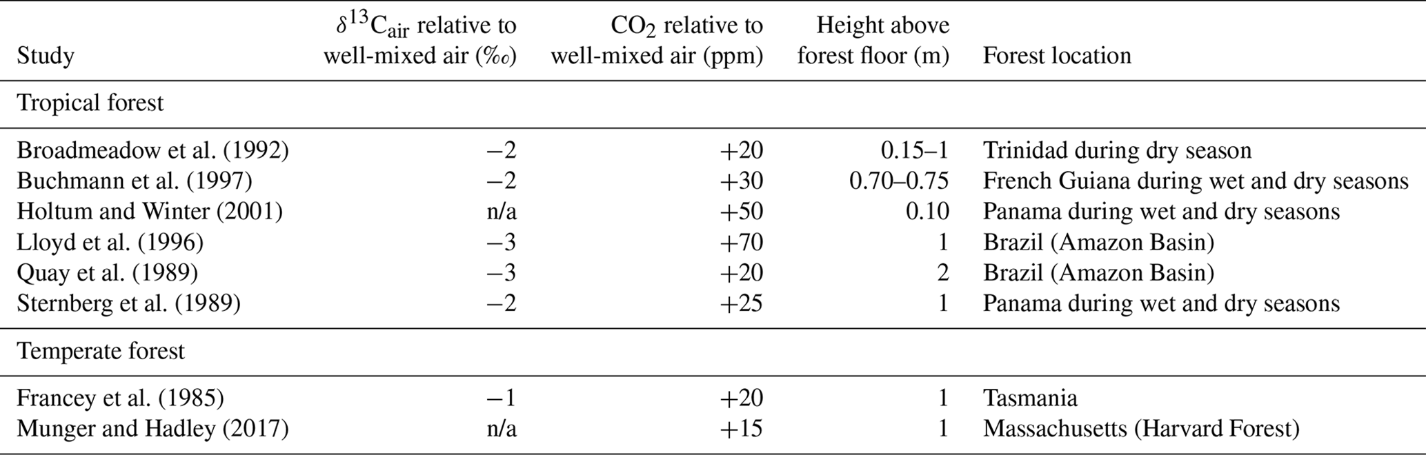
n/a: not applicable
As a result, leaves that grow close to the forest floor may cause the Franks model to produce CO2 estimates higher than that of the mixed atmosphere for at least two reasons. First, the concentration of CO2 near the forest floor is elevated; that is, the model may correctly estimate a CO2 concentration that the user is not interested in. Second, because the δ13Cair that a forest-floor plant experiences is lower than the global well-mixed value, if the user chooses the well-mixed value for model input (inferred, for example, from the δ13C of marine carbonate; Tipple et al., 2010), then ci∕ca and thus atmospheric CO2 will be overestimated (see Eq. 2).
We sought to test how the Franks model is affected by the forest-floor microenvironment for five tropical angiosperm species and 15 temperate angiosperm and fern species. The tropical leaves were sampled at ∼1–2 m of height from Parque Nacional San Lorenzo, Panama. In contrast to the canopy dataset from San Lorenzo (Sect. 2.1), these CO2 estimates have not been previously reported. In the summer of 2015, seven fern species were sampled at ∼0.5 m of height from Connecticut College and Wesleyan University. Also, we used leaf vouchers from Royer et al. (2010), who sampled eight herbaceous angiosperm species at ∼0.1–0.2 m of height from Reed Gap, Connecticut. For all 20 species, stomatal and carbon isotopic measurements follow the methods described in Sect. 2.1. Table S1 contains all of the inputs needed to run the Franks model, along with the estimated CO2 concentrations.
We also investigated if we could include the forest-floor δ13Cair effect in our estimates of atmospheric CO2. We did not measure the CO2 concentration and δ13Cair around our plants, so we could not directly compare our values. But, if the only CO2 inputs close to the forest floor are from the soil and well-mixed atmosphere, then the system can be modeled as a two-end-member mixing model in which δ13Cair has a positive, linear relationship with 1∕CO2 (Keeling, 1958). If the CO2 concentration and δ13C of both end-members are known, the forest-floor microenvironment should fall somewhere on the modeled line. Importantly, the Franks model provides a second constraint on the system. Here, δ13Cair has a negative, nonlinear relationship with 1∕CO2 because δ13Cair is positively related to ci∕ca and CO2. The Franks model thus provides a second calculation for the relationship between δ13Cair and estimated CO2 concentration. The intersection between the two curves should be the correct δ13Cair and CO2 concentration for the forest-floor microenvironment.
To estimate the soil CO2 end-member, we measured the δ13C of soil organic matter collected from the A horizons of 13 soil sites at San Lorenzo and of five each at Reed Gap and Connecticut College. For all soils, we assume a 5000 ppm CO2 concentration for a depth that is below the zone of CO2 diffusion from the atmosphere (∼0.3 m; Cerling, 1999; Breecker et al., 2009). The true value for wet temperate and tropical forest soils may be somewhat less or substantially more than 5000 ppm (Medina et al., 1986; Cerling, 1999; Hirano et al., 2003; Hashimoto et al., 2004; Sotta et al., 2004). Because the mixing model uses 1∕CO2, a much higher CO2 concentration (e.g., 10 000 ppm) has little impact on our results.
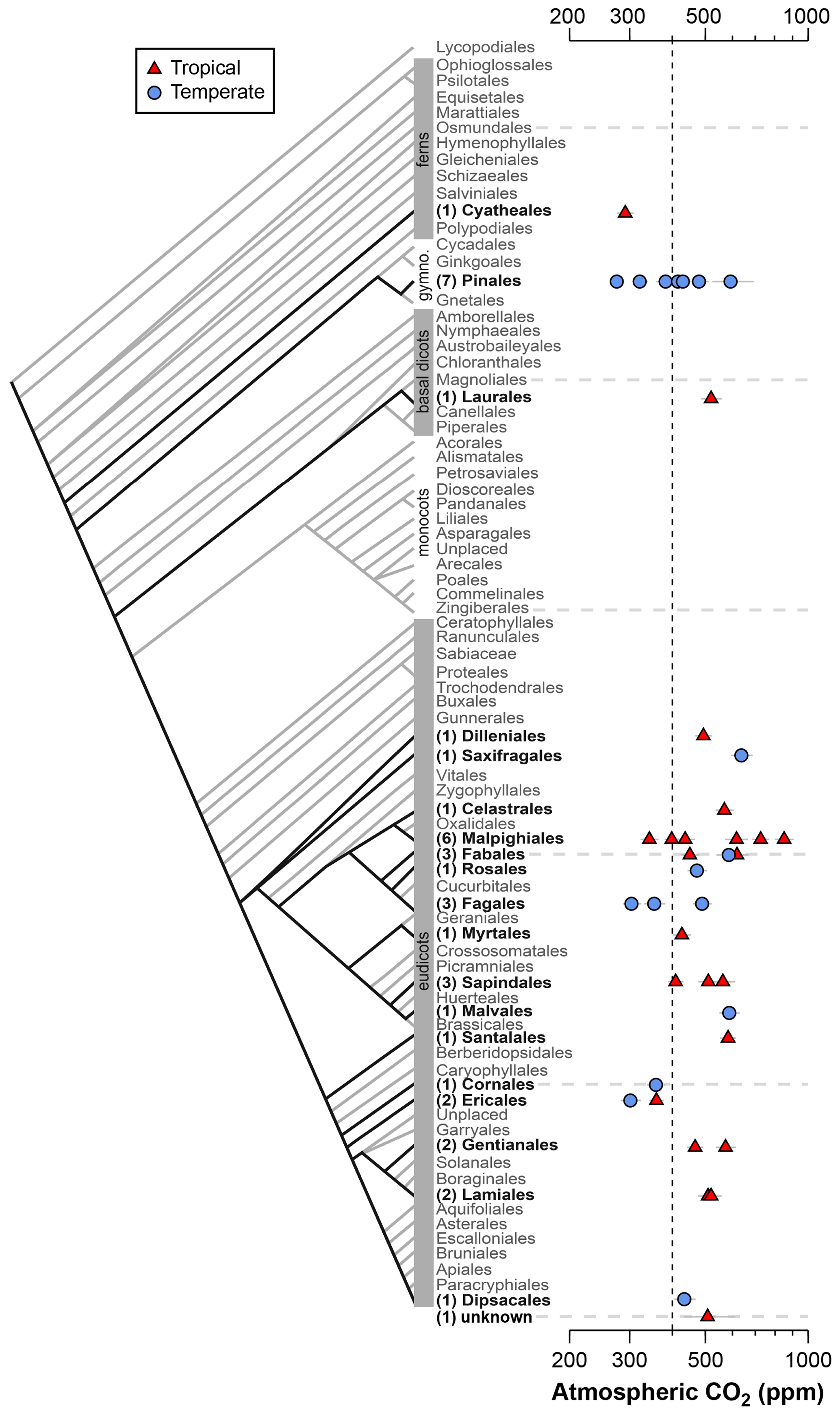
Figure 2Estimates of CO2 based on canopy leaves from 40 tree species. Uncertainties in the estimates correspond to the 16th–84th percentile range. Vertical line is the correct concentration (400 ppm). On the left is an order-level vascular plant phylogeny (APW v.13; Stevens, 2001, onwards). The number of measured species is given in parentheses.
3.1 General testing in living plants
Estimates of CO2 across the 40 tree species sampled in the field range from 275 to 850 ppm, with a mean of 478 ppm and median of 472 ppm (Fig. 2); two-thirds of the estimates (a close equivalent to ±1 standard deviation) range between 353 and 585 ppm. In 28 % of the tested species, the estimated CO2 concentrations overlap the target concentration (400 ppm) at 95 % confidence; for these species, the CO2 estimates do not differ significantly from the target. There are no strong differences across taxonomic orders or between leaves from tropical and temperate forests. The mean error rate across the estimates is 28 % (median 24 %), which is higher than estimates that include direct measurements of the physiological inputs A0 and gc(op)∕gc(max) (mean 20 %; median 13 %; Fig. 1). Along similar lines, if the estimates presented in Fig. 1 are reestimated using the values for A0 and gc(op)∕gc(max) recommended by Franks et al. (2014), the mean error rate increases to 37 % (median 33 %). If only the default values of A0 are used, the median error rate is 27 %, and for only default values of gc(op)∕gc(max) it is 22 %.
These results indicate that CO2 accuracy is generally improved when A0 and/or gc(op)∕gc(max) are measured. These measurements require expensive gas-exchange equipment and are not always easy or practical to make. Moreover, A0 and gc(op)∕gc(max) cannot be measured on fossils. Some gains in accuracy are possible by measuring A0 and gc(op)∕gc(max) on extant relatives of the fossil species (e.g., the same genus). Absent of this, our analysis using the recommended mean values of Franks et al. (2014) indicates an error rate, on average, of approximately 28 %. This is comparable to or better than other leading paleo-CO2 proxies (Franks et al., 2014).
One reliable way to improve accuracy is to estimate CO2 with multiple species because the falsely high and falsely low estimates partly cancel each other out. The grand mean of estimates presented in Fig. 2 (478 ppm) is 20 % from the 400 ppm target, which is less than the 28 % mean error rate of individual estimates.
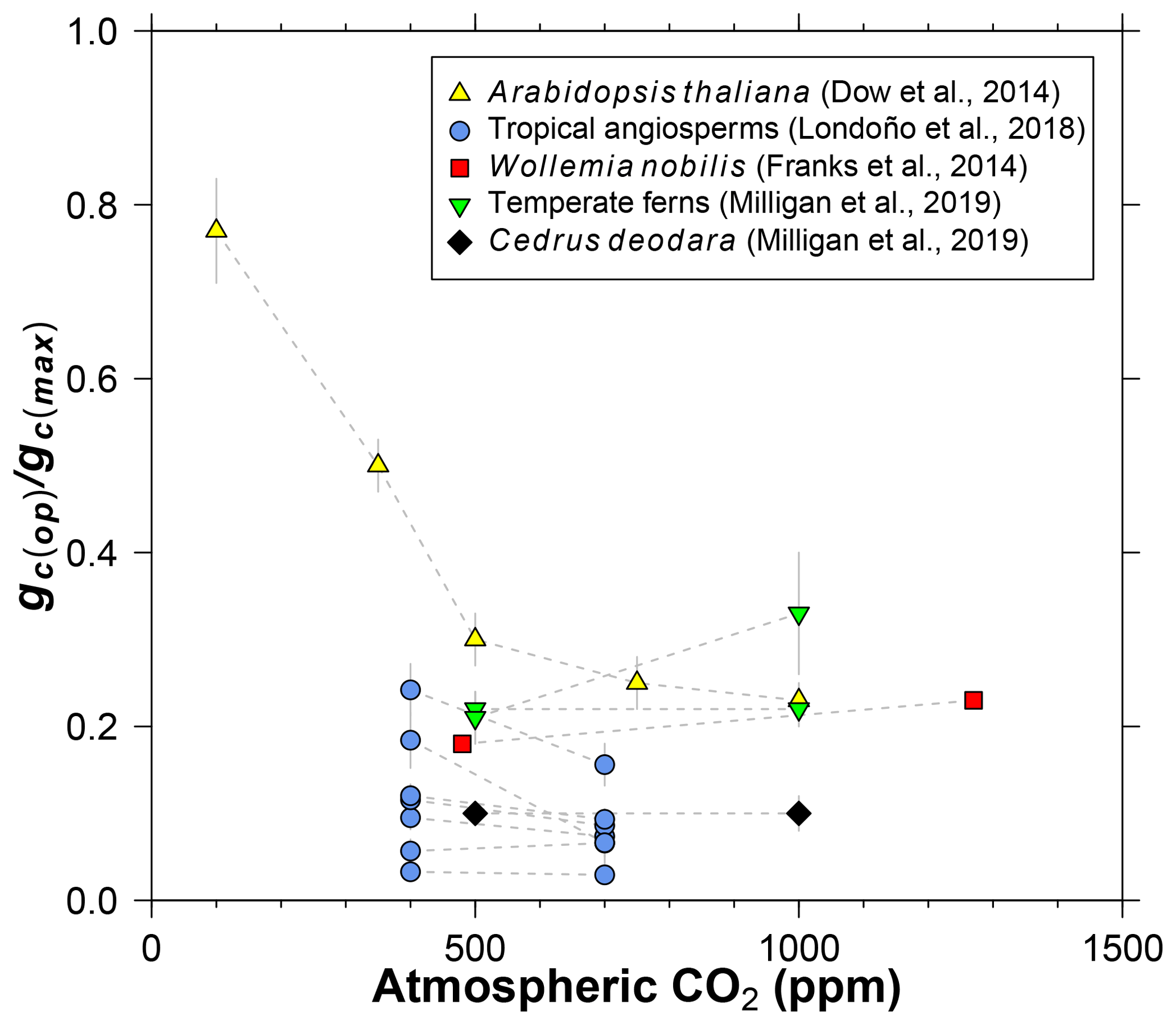
Figure 3Literature compilation of the sensitivity of gc(op)∕gc(max) (ratio of operational to maximum leaf conductance to CO2) to atmospheric CO2 concentration.
Dow et al. (2014) observed that gc(op)∕gc(max) inversely varies with CO2 in Arabidopsis thaliana, but primarily at subambient concentrations (yellow triangles in Fig. 3). At elevated CO2, gc(op)∕gc(max) is close to 0.2, which is the value recommended by Franks et al. (2014). Data from 11 species of angiosperms, conifers, and ferns at present-day (or near present-day) and elevated CO2 concentrations support the view of a limited effect at high CO2 (Fig. 3; Franks et al., 2014; Londoño et al., 2018; Milligan et al., 2019). More data at subambient CO2 are needed, but for CO2 concentrations similar to or higher than the present day, we see no strong reason to include a CO2 sensitivity in gc(op)∕gc(max). The rather low values for Cedrus deodara and many of the tropical angiosperms (<0.1) are likely due to stress imposed by their growth-chamber environment; these gc(op)∕gc(max) values are probably not representative of field-grown trees, which tend to be closer to 0.2 (Franks et al., 2014).
3.2 Temperature
The temperature sensitivities of the ratio of diffusivity of CO2 in air to the molar volume of air (d∕v) and the CO2 compensation point in the absence of dark respiration (Γ*) have little effect on estimated CO2 in the Franks model (Fig. 4). Given that assimilation-weighted leaf temperature only varies about 7 ∘C across plants today, the differences shown in Fig. 4, which are based on leaf temperatures of 25 and 15 ∘C, are likely a maximum effect. As such, we consider the use of a fixed leaf temperature (e.g., 25 ∘C) in the model to be a defensible simplification.
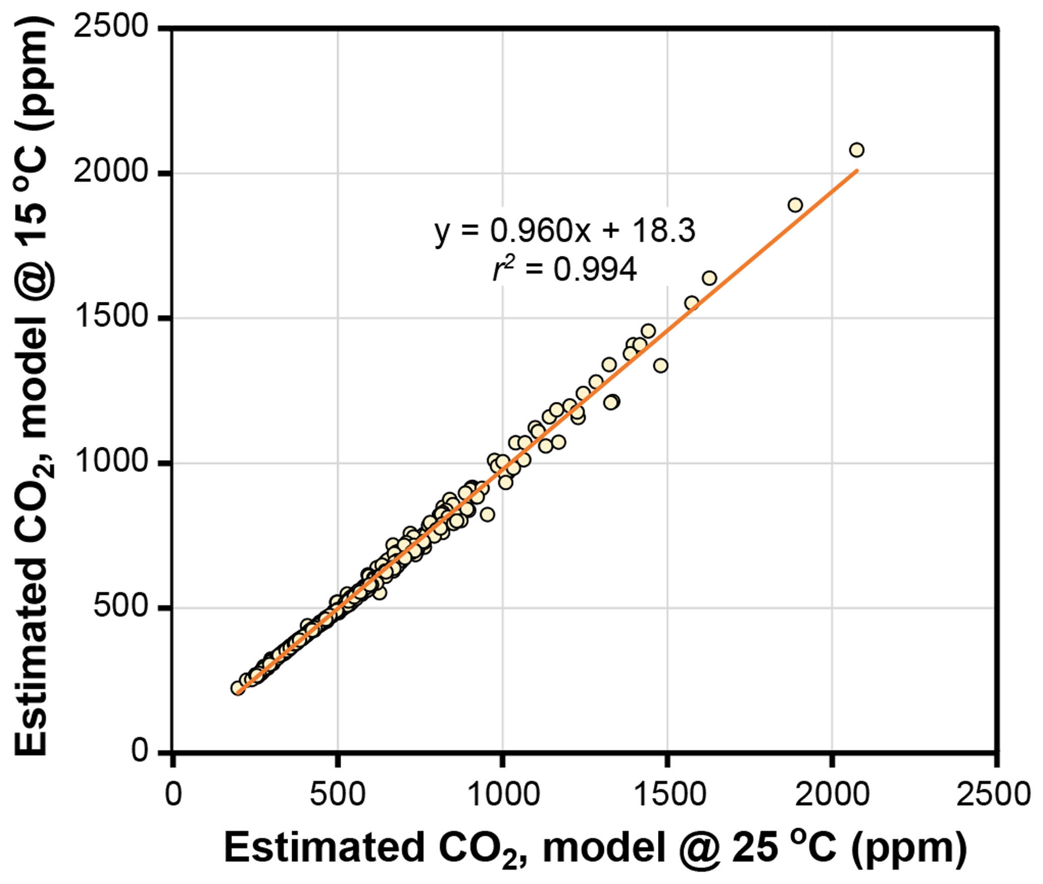
Figure 4Estimates of CO2 at leaf temperatures of 25 ∘C and 15 ∘C. Each symbol is an extant or fossil leaf. The difference in estimated CO2 for any leaf is due to the theoretical effects of temperature on gas diffusion (d∕v) and the CO2 compensation point in the absence of dark respiration (Γ*) (Eqs. 6–8).
Other inputs in the model may respond to temperature, though. In our growth-chamber experiments for which daytime air temperatures were 28 and 20 ∘C, the effect on estimated CO2 was mixed (Fig. 5). In five out of six species, estimated CO2 was higher in the warm treatment, but for all species these differences were not statistically significant (p>0.05 based on a KS test; see Methods). Incorporating the temperature sensitivities in d∕v and Γ* had little effect (“adj” estimates in Fig. 5), as expected from Fig. 4.
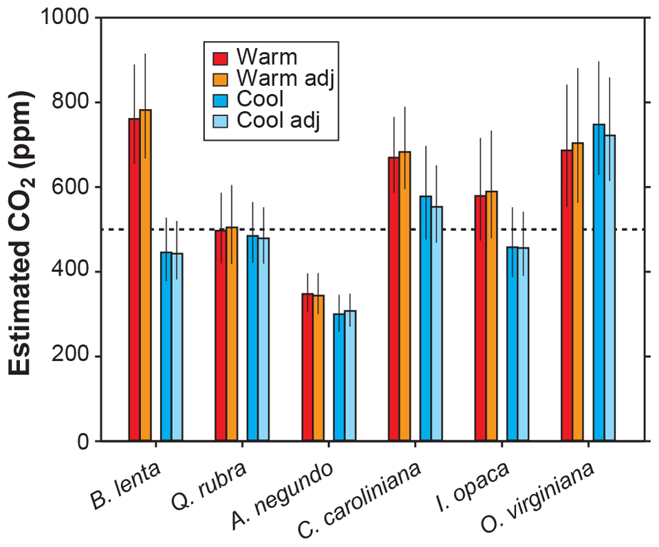
Figure 5Estimates of CO2 for plants grown inside growth chambers at daytime air temperatures of 28 and 20 ∘C. Also shown are estimates after taking into account the temperature sensitivity of gas diffusion (d∕v) and the CO2 compensation point in the absence of dark respiration (Γ*) (“adj”; see also Fig. 4). Dashed line is the correct CO2 concentration (500 ppm). Uncertainties in the estimates correspond to the 16th–84th percentile range.
None of the measured inputs – stomatal density, stomatal pore length, single guard cell width, and leaf δ13C – were significantly affected by temperature across all species (p>0.05 for each of the four inputs based on a mixed model; see Sect. 2.2). These small differences probably cannot account for the differences in estimated CO2 between temperatures. It is more likely that some of the inputs that we did not directly measure, such as assimilation rate (A0), the gc(op)∕gc(max) ratio, or mesophyll conductance (gm), differ from the true mean value. In the cases for the five species for which estimated CO2 is higher in the warm treatment, our mean A0 for the warm plants must be falsely high, or gc(op)∕gc(max) or gm is falsely low.
In summary, we see no strong reason to expand the parameterization of temperature in the model, though more growth-chamber experiments may be warranted. We note that in three out of the six species from the warm treatment, the estimated CO2 cannot be distinguished from the 500 ppm target at 95 % confidence; for the cool treatment, this is true for four of the species. Also, the across-species means of estimated CO2 for the warm and cool treatments are reasonably close to the target (590 and 502 ppm, respectively) and overall have a mean error rate of 25 %. This level of uncertainty is similar to our field estimates for which we did not measure A0 or gc(op)∕gc(max) (28 %; see Fig. 2). This too provides support for our recommendation that it is not critical to include a broader treatment of temperature in the model.
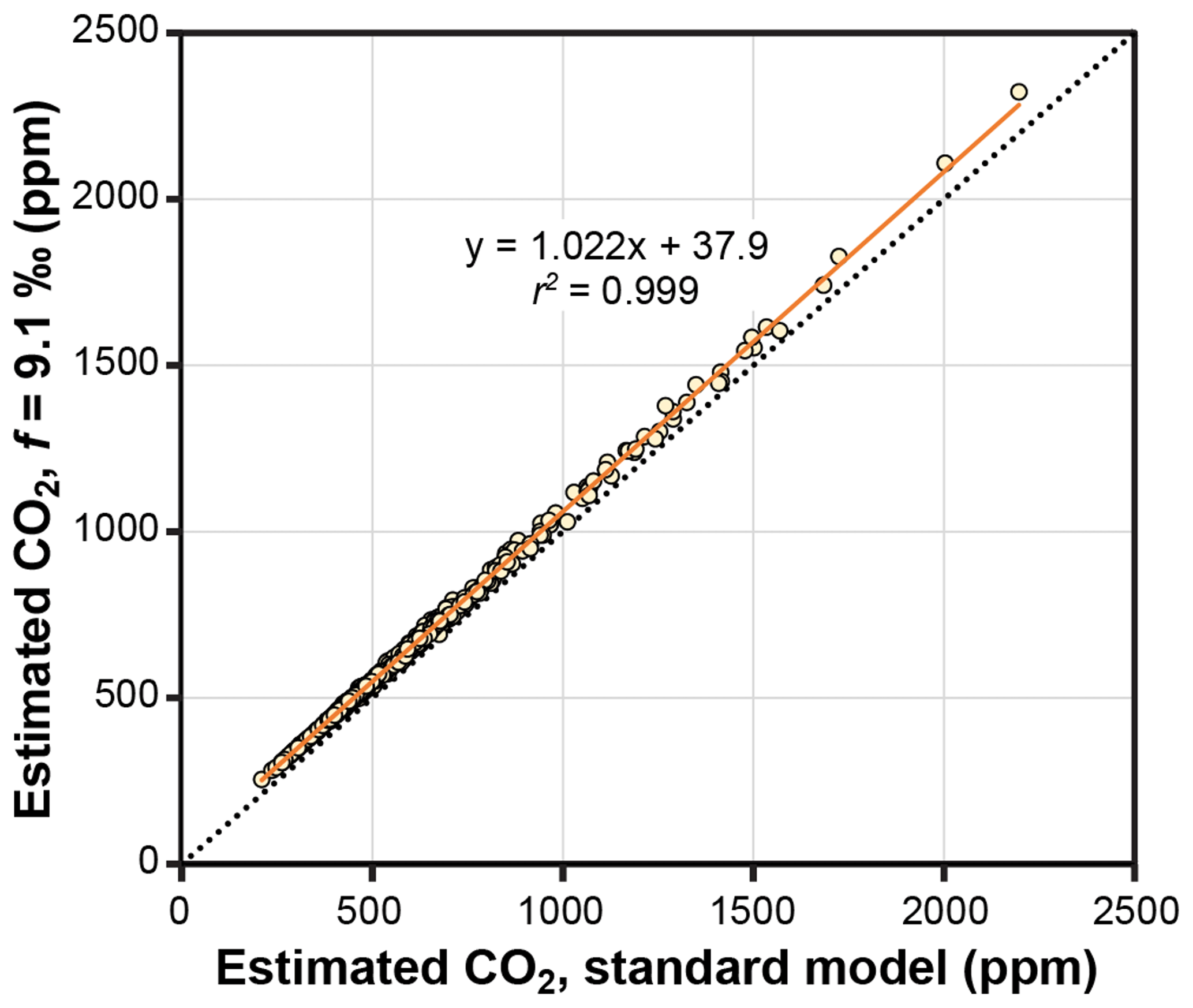
Figure 6Estimates of CO2 with and without a photorespiration effect (f=9.1 ‰; see Eq. 10). Each symbol is an extant or fossil leaf. Dashed line is y=x.
3.3 Photorespiration
The theoretical effects of photorespiration do not strongly impact estimates of CO2 in the Franks model. The average effect for our 409 extant and fossil leaves is to increase estimated CO2 by 2.2 % plus 38 ppm (Fig. 6). At 1000 ppm, for example, estimates would increase by 60 ppm. This calculation assumes a photorespiration fractionation (f) of 9.1 ‰, which is the value estimated for Arabidopsis thaliana (Schubert and Jahren, 2018). If a fractionation towards the upper bound of published estimates is used instead (15 ‰), estimated CO2 increases on average by 3.8 % plus 61 ppm. Across this range in f, the associated uncertainty in estimated CO2 is well within the method's overall precision ( % at 95 % confidence; Franks et al., 2014). As such, CO2 estimates made without these photorespiration effects (i.e., using Eq. 9 instead of Eq. 10) should be reliable, although some improvement is possible using Eq. 10 in cases in which f is accurately known.
We note that both f and Γ* are also affected by atmospheric O2 concentration. Because O2 is directly responsible for photorespiration, f should scale with O2 (or, more precisely, the O2 : CO2 molar ratio). Unfortunately, this effect is poorly constrained (Beerling et al., 2002; Berner et al., 2003; Porter et al., 2017). In contrast, the theoretical effect of O2 on Γ* is known: it is linear with an approximate slope of 2 (Farquhar et al., 1982; see their Eq. B13). During the Phanerozoic, O2 likely ranged from 10 % to 30 %, with lows during the early Paleozoic and early Triassic and highs during the Carboniferous to early Permian and Cretaceous (Berner, 2009; Glasspool and Scott, 2010; Arvidson et al., 2013; Mills et al., 2016; Lenton et al., 2018). Assuming a present-day Γ* of 40 ppm (at 21 % O2), Γ* would be 60 ppm at 30 % O2 and 20 ppm at 10 % O2. Running the Franks model on our library of 409 extant and fossil leaves, we find little effect on estimated CO2: estimates are 7.4 % higher on average at 30 % O2 than at 10 % O2 (see also McElwain et al., 2016).
3.4 Leaves that grow close to the forest floor
CO2 estimates for tropical understory leaves from five species at San Lorenzo, Panama, are very high, ranging from 1903 to 18863 ppm (species mean 6837 ppm). For two of the species, Londoño et al. (2018) also analyzed canopy leaves from trees nearby, and these within-species comparisons highlight the vast discrepancy (Ocotea sp.: 541 vs. 5737 ppm; Tontelea sp.: 622 vs. 18 863 ppm). The primary difference in the inputs between the canopy and understory leaves is the δ13Cleaf: Londoño et al. (2018) report a species mean δ13Cleaf of −30.0 ‰ for the 21 canopy species versus −35.6 ‰ for the five understory species. This difference leads to very different mean estimates of ci∕ca: 0.69 for canopy leaves versus a highly unrealistic (Diefendorf et al., 2010) 0.93 for understory leaves.
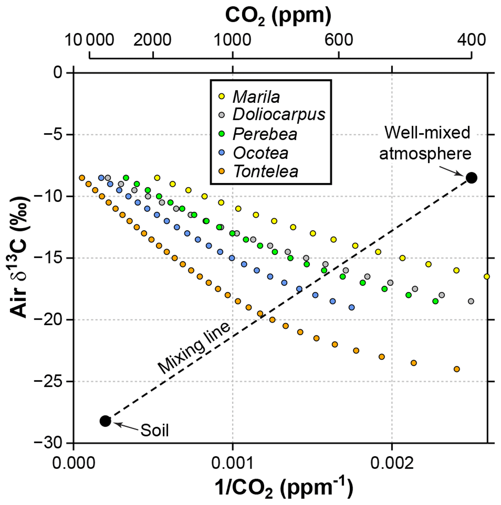
Figure 7Sensitivity of estimated CO2 in the Franks model to the δ13C of atmospheric CO2. Estimates come from leaves of five angiosperm species that grew close to the forest floor in Parque Nacional San Lorenzo, Panama. For each species, the step in δ13Cair between estimates is 0.5 ‰. The dashed line is a two-end-member mixing model for CO2 between the soil and well-mixed atmosphere. The intersection between the mixing model and the Franks model should correspond to the CO2 concentration and δ13Cair of the forest-floor microenvironment.
It is likely that the high CO2 estimates from understory leaves are mostly driven by falsely high δ13Cair inputs. Following the mixing model strategy outlined in Sect. 2.4 (and based on a soil organic matter δ13C of −28.2 ‰ measured at San Lorenzo), we calculate a species mean δ13Cair of −16.7 ‰ (mean of intersection points in Fig. 7). When this δ13Cair is used to estimate CO2 with the Franks model (instead of −8.5 ‰), the species mean drops to 699 ppm. This is somewhat higher than the species mean from canopy leaves in the same forest (563 ppm; red triangles in Fig. 2; Londoño et al., 2018).
Understory leaves from Connecticut temperate forests show similar but less dramatic patterns, which we attribute to a more open canopy with stronger atmospheric mixing. CO2 estimates for the 15 species range from 447 to 1567 ppm (mean 794 ppm). Our intersection method identifies a mean δ13Cair of −11.2 ‰ for the Wesleyan and Connecticut College campuses (based on a soil δ13C of −27.6 ‰ measured at Connecticut College) and −10.3 ‰ for Reed Gap (soil δ13C ‰). Using these adjusted δ13Cair, the species mean of estimated CO2 drops to 566 ppm, which is somewhat higher than the species mean from canopy leaves in the same areas (449 ppm; blue circles in Fig. 2).
We acknowledge that this analysis is too simple. First, we did not measure the understory CO2 concentration and δ13Cair (this would require repeated measurements during different daytime hours over a growing season to calculate a time-integrated value); instead, we assumed a simple two-end-member mixing model between the soil and well-mixed atmosphere. Second, other factors probably contribute to the differences in estimated CO2 between canopy and understory leaves. Our predicted δ13Cair values are too low (∼8 ‰ and 2 ‰ lower than the well-mixed atmosphere for the tropical and temperate forests) and our estimated CO2 too high (∼100 ppm higher than that from canopy leaves). In the lowermost 1–2 m of the canopy, previous work suggests up to a −3 ‰ and +70 ppm deviation in tropical forests and −1 ‰ ∕ +20 ppm in temperate forests (Table 1). One input that could help to resolve this discrepancy is the assimilation rate (A0). We assumed a fixed A0 of 12 µmol m−2 s−1 for all leaves, regardless of canopy position. Shade leaves often have lower assimilation rates than sun leaves (Givnish, 1988). Substituting lower A0 values for understory leaves would lower estimated CO2 roughly in proportion (Eqs. 2–3). Using lower A0 values for shade leaves in the model is appropriate, but determining the best value is difficult. Typical A0 values for leaves growing at the top of the canopy in full sun are far more consistent because photosynthesis in these leaves is usually at its maximum capacity (saturated at full sunlight) for the prevailing atmospheric CO2 concentration. Because the degree of shadiness near the forest floor is highly variable, photosynthesis (A0) in these leaves will be acclimated to some fraction of the full-sun maximum in a sun-exposed leaf, but careful thought must go into determining what this fraction is.
We note that our mixing model strategy cannot be applied to fossils because the global atmospheric CO2 concentration is needed (one end point for dashed line in Fig. 7). Instead, our motivation for the analysis is to demonstrate that (1) leaves growing in the lowermost 2 m of the canopy should be considered with caution in the context of the Franks model, and (2) the failure of the model is due to faulty inputs (mostly δ13Cair), not the model itself.
In most fossil leaf deposits, shade morphotypes are comparatively rare (e.g., Kürschner, 1997; Wang et al., 2018) because – relative to sun leaves – they are less durable, do not travel as far by wind, and are produced at a slower rate (Dilcher, 1973; Roth and Dilcher, 1978; Spicer, 1980; Ferguson, 1985; Burnham et al., 1992). Our recommendation is to exclude such leaves. There are several ways to differentiate sun vs. shade morphotypes: overall shape (Talbert and Holch, 1957; Givnish, 1978; Kürschner, 1997; Sack et al., 2006), shape of epidermal cells (larger and with a more undulated outline in shade leaves; Kürschner, 1997; Dunn et al., 2015), vein density (lower in shade leaves; Uhl and Mosbrugger, 1999; Sack and Scoffoni, 2013; Crifò et al., 2014; Londoño et al., 2018), and range in δ13Cleaf (high when both sun and shade leaves are present, for example in our study; Graham et al., 2014). Not all shade leaves grow within 2 m of the forest floor, but excluding all such leaves would eliminate the forest-floor bias.
The Franks model is reasonably accurate (∼28 % error rate) even when the physiological inputs A0 (assimilation rate at a known CO2 concentration) and gc(op)∕gc(max) (ratio of operational to maximum leaf conductance to CO2) are inferred, not measured. Accuracy does improve when these inputs are measured (∼20 % error rate), but such measurements are not possible with fossils and may not always be feasible with the nearest living relatives. A 28 % error rate is broadly in line with (or better than) other leading paleo-CO2 proxies.
Most of the possible confounding factors that we investigated appear minor. The temperature sensitivities of d∕v (related to gas diffusion) and Γ* (CO2 compensation point in the absence of dark respiration) have a negligible impact on estimated CO2. Our temperature experiments in growth chambers point to larger differences in some species, which must be related to incorrect values for inputs that were not directly measured, such as A0, gc(op)∕gc(max), and gm (mesophyll conductance). Overall, though, we find that the differences in estimated CO2 imparted by temperature are generally smaller than the overall 28 % error rate.
Incorporating the covariance between CO2 concentration and photorespiration leads to only small changes in estimated CO2. O2 concentration affects photorespiration and may thus confound CO2 estimates from the Franks model, but presently the effect is poorly quantified. The effect of O2 on Γ* is better known and imparts only small changes in estimated CO2 across a feasible range in Phanerozoic O2 of 10 %–30 %.
Leaves from the lowermost 1–2 m of the canopy experience slightly elevated CO2 concentrations and lower air δ13C during the daytime relative to the well-mixed atmosphere. We find that if we use the well-mixed air δ13C to estimate CO2 from leaves that grew near the forest floor, estimates are too high, especially in dense tropical canopies. When we use a two-end-member mixing model to calculate the correct local air δ13C, the falsely high CO2 estimates largely disappear. For fossil applications, shade leaves from the bottom of the canopy should be avoided. Shade leaves are typically rare in the fossil record (relative to sun leaves) and can be identified by their overall shape, the shape of their epidermal cells, their low leaf δ13C, and their low vein density.
Conceptually, the Franks model holds considerable promise for quantifying paleo-CO2: it is mechanistically grounded and can be applied to most fossil leaves. Our tests of the model's accuracy and sensitivity to temperature and photorespiration largely uphold this promise.
All new data are presented in the Supplement.
The supplement related to this article is available online at: https://doi.org/10.5194/cp-15-795-2019-supplement.
DR, KM, MM, and LL designed and conducted the experiments; all authors interpreted the data; DR prepared the paper with contributions from all coauthors.
The authors declare that they have no conflict of interest.
We thank Glenn Dreyer and Peter Siver for logistical support at Connecticut College, Shuo Wang for lab assistance, and Camilla Crifò and Andres Baresh for collecting the tropical samples. Support for LL was provided by the Smithsonian Tropical Research Institute, the Mark Tupper Fellowship, the National Science Foundation (grants EAR 0824299 and OISE, EAR, DRL 0966884), the Anders Foundation, and Gregory D. and Jennifer Walston Johnson and the 1923 Fund.
This paper was edited by Ed Brook and reviewed by Jennifer Mc Elwain and one anonymous referee.
Arvidson, R. S., Mackenzie, F. T., and Guidry, M. W.: Geologic history of seawater: A MAGic approach to carbon chemistry and ocean ventilation, Chem. Geol., 362, 287–304, https://doi.org/10.1016/j.chemgeo.2013.10.012, 2013.
Barclay, R. S. and Wing, S. L.: Improving the Ginkgo CO2 barometer: implications for the early Cenozoic atmosphere, Earth Planet. Sci. Lett., 439, 158–171, https://doi.org/10.1016/j.epsl.2016.01.012, 2016.
Bates, D., Mächler, M., Bolker, B., and Walker, S.: Fitting linear mixed-effects models using lme4, J. Stat. Softw., 67, 1–48, https://doi.org/10.18637/jss.v067.i01, 2015.
Beerling, D. J.: Evolutionary responses of land plants to atmospheric CO2, in: A History of Atmospheric CO2 and Its Effects on Plants, Animals, and Ecosystems, edited by: Ehleringer, J. R., Cerling, T. E., and Dearing, M. D., Springer, New York, 114–132, 2005.
Beerling, D. J., Fox, A., and Anderson, C. W.: Quantitative uncertainty analyses of ancient atmospheric CO2 estimates from fossil leaves, Am. J. Sci., 309, 775–787, https://doi.org/10.2475/09.2009.01, 2009.
Beerling, D. J., Lake, J. A., Berner, R. A., Hickey, L. J., Taylor, D. W., and Royer, D. L.: Carbon isotope evidence implying high O2∕CO2 ratios in the Permo-Carboniferous atmosphere, Geochimica et Cosmochimica Acta, 66, 3757–3767, https://doi.org/10.1016/S0016-7037(02)00901-8, 2002.
Bernacchi, C. J., Pimentel, C., and Long, S. P.: In vivo temperature response functions of parameters required to model RuBP-limited photosynthesis, Plant Cell Environ., 26, 1419–1430, https://doi.org/10.1046/j.0016-8025.2003.01050.x, 2003.
Berner, R. A.: Phanerozoic atmospheric oxygen: new results using the GEOCARBSULF model, Am. J. Sci., 309, 603-606, https://doi.org/10.2475/07.2009.03, 2009.
Berner, R. A., Beerling, D. J., Dudley, R., Robinson, J. M., and Wildman, R. A.: Phanerozoic atmospheric oxygen, Annu. Rev. Earth Pl Sc., 31, 105–134, https://doi.org/10.1146/annurev.earth.31.100901.141329, 2003.
Breecker, D. O., Sharp, Z. D., and McFadden, L. D.: Seasonal bias in the formation and stable isotopic composition of pedogenic carbonate in modern soils from central New Mexico, USA, Geol. Soc. Am. Bull., 121, 630–640, https://doi.org/10.1130/B26413.1, 2009.
Broadmeadow, M., Griffiths, H., Maxwell, C., and Borland, A.: The carbon isotope ratio of plant organic material reflects temporal and spatial variations in CO2 within tropical forest formations in Trinidad, Oecologia, 89, 435–441, https://doi.org/10.1007/BF00317423, 1992.
Buchmann, N., Guehl, J.-M., Barigah, T., and Ehleringer, J. R.: Interseasonal
comparison of CO2 concentrations, isotopic composition, and carbon
dynamics in an Amazonian rainforest (French Guiana), Oecologia, 110, 120–131,
doi10.1007/s004420050140, 1997.
Burnham, R. J., Wing, S. L., and Parker, G. G.: The reflection of deciduous forest communities in leaf litter: implications for autochthonous litter assemblages from the fossil record, Paleobiology, 18, 30–49, https://doi.org/10.1017/S0094837300012203, 1992.
Cerling, T. E.: Stable carbon isotopes in palaeosol carbonates, Special Publications of the International Association of Sedimentologists, 27, 43–60, 1999.
Chaloner, W. G. and McElwain, J.: The fossil plant record and global climatic change, Rev. Palaeobot. Palyno., 95, 73–82, https://doi.org/10.1016/S0034-6667(96)00028-0, 1997.
Crifò, C., Currano, E. D., Baresch, A., and Jaramillo, C.: Variations in angiosperm leaf vein density have implications for interpreting life form in the fossil record, Geology, 42, 919–922, https://doi.org/10.1130/g35828.1, 2014.
Diefendorf, A. F., Mueller, K. E., Wing, S. L., Koch, P. L., and Freeman, K. H.: Global patterns in leaf 13C discrimination and implications for studies of past and future climate, P. Natl. Acad. Sci. USA, 107, 5738–5743, https://doi.org/10.1073/pnas.0910513107, 2010.
Dilcher, D. L.: A paleoclimatic interpretation of the Eocene floras of southeastern North America, in: Vegetation and Vegetational History of Northern Latin America, edited by: Graham, A., Elsevier, Amsterdam, 39–53, 1973.
Doria, G., Royer, D. L., Wolfe, A. P., Fox, A., Westgate, J. A., and Beerling, D. J.: Declining atmospheric CO2 during the late Middle Eocene climate transition, Am. J. Sci., 311, 63–75, https://doi.org/10.2475/01.2011.03, 2011.
Dow, G. J., Bergmann, D. C., and Berry, J. A.: An integrated model of stomatal development and leaf physiology, New Phytol., 201, 1218–1226, https://doi.org/10.1111/nph.12608, 2014.
Dunn, R. E., Strömberg, C. A. E., Madden, R. H., Kohn, M. J., and Carlini, A. A.: Linked canopy, climate, and faunal change in the Cenozoic of Patagonia, Science, 347, 258–261, https://doi.org/10.1126/science.1260947, 2015.
Erdei, B., Utescher, T., Hably, L., Tamás, J., Roth-Nebelsick, A., and Grein, M.: Early Oligocene continental climate of the Palaeogene Basin (Hungary and Slovenia) and the surrounding area, Turk. J. Earth Sci., 21, 153–186, https://doi.org/10.3906/yer-1005-29, 2012.
Farquhar, G., von Caemmerer, S., and Berry, J.: A biochemical model of photosynthetic CO2 assimilation in leaves of C3 species, Planta, 149, 78–90, https://doi.org/10.1007/BF00386231, 1980.
Farquhar, G. D. and Sharkey, T. D.: Stomatal conductance and photosynthesis, Ann. Rev. Plant Physio., 33, 317–345, https://doi.org/10.1146/annurev.pp.33.060182.001533, 1982.
Farquhar, G. D., O'Leary, M. H., and Berry, J. A.: On the relationship between carbon isotope discrimination and the intercellular carbon dioxide concentration in leaves, Aust. J. Plant Physiol., 9, 121–137, https://doi.org/10.1071/PP9820121, 1982.
Ferguson, D. K.: The origin of leaf-assemblages – new light on an old problem, Rev. Palaeobot. Palyno, 46, 117–188, https://doi.org/10.1016/0034-6667(85)90041-7, 1985.
Francey, R., Gifford, R., Sharkey, T., and Weir, B.: Physiological influences on carbon isotope discrimination in huon pine (Lagarostrobos franklinii), Oecologia, 66, 211–218, https://doi.org/10.1007/BF00379857, 1985.
Franks, P. J., Leitch, I. J., Ruszala, E. M., Hetherington, A. M., and Beerling, D. J.: Physiological framework for adaptation of stomata to CO2 from glacial to future concentrations, Philos. T. R. Soc. B, 367, 537–546, https://doi.org/10.1098/rstb.2011.0270, 2012.
Franks, P. J., Royer, D. L., Beerling, D. J., Van de Water, P. K., Cantrill, D. J., Barbour, M. M., and Berry, J. A.: New constraints on atmospheric CO2 concentration for the Phanerozoic, Geophys. Res. Lett., 41, 4685–4694, https://doi.org/10.1002/2014gl060457, 2014.
Givnish, T. J.: Ecological aspects of plant morphology: leaf form in relation to environment, Acta Biotheor., 27, 83–142, 1978.
Givnish, T. J.: Adaptation to sun and shade: a whole-plant perspective, Aust. J. Plant Physiol., 15, 63–92, https://doi.org/10.1071/PP9880063, 1988.
Glasspool, I. J. and Scott, A. C.: Phanerozoic concentrations of atmospheric oxygen reconstructed from sedimentary charcoal, Nat. Geosci., 3, 627–630, https://doi.org/10.1038/ngeo923, 2010.
Graham, H. V., Patzkowsky, M. E., Wing, S. L., Parker, G. G., Fogel, M. L.,
and Freeman, K. H.: Isotopic characteristics of canopies in simulated leaf
assemblages, Geochim. Cosmochim. Ac., 144, 82–95,
doi10.1016/j.gca.2014.08.032, 2014.
Grein, M., Utescher, T., Wilde, V., and Roth-Nebelsick, A.: Reconstruction of the middle Eocene climate of Messel using palaeobotanical data, Neues. Jahrb. Geol. P.-A., 260, 305–318, https://doi.org/10.1127/0077-7749/2011/0139, 2011a.
Grein, M., Konrad, W., Wilde, V., Utescher, T., and Roth-Nebelsick, A.: Reconstruction of atmospheric CO2 during the early Middle Eocene by application of a gas exchange model to fossil plants from the Messel Formation, Germany, Palaeogeogr. Palaeocl., 309, 383–391, https://doi.org/10.1016/j.palaeo.2011.07.008, 2011b.
Grein, M., Oehm, C., Konrad, W., Utescher, T., Kunzmann, L., and Roth-Nebelsick, A.: Atmospheric CO2 from the late Oligocene to early Miocene based on photosynthesis data and fossil leaf characteristics, Palaeogeogr. Palaeocl., 374, 41–51, https://doi.org/10.1016/j.palaeo.2012.12.025, 2013.
Hashimoto, S., Tanaka, N., Suzuki, M., Inoue, A., Takizawa, H., Kosaka, I., Tanaka, K., Tantasirin, C., and Tangtham, N.: Soil respiration and soil CO2 concentration in a tropical forest, Thailand, J. For. Res.-Jpn., 9, 75–79, https://doi.org/10.1007/s10310-003-0046-y, 2004.
Haworth, M., Heath, J., and McElwain, J. C.: Differences in the response sensitivity of stomatal index to atmospheric CO2 among four genera of Cupressaceae conifers, Ann. Bot.-London, 105, 411–418, https://doi.org/10.1093/aob/mcp309, 2010.
Helliker, B. R. and Richter, S. L.: Subtropical to boreal convergence of tree-leaf temperatures, Nature, 454, 511–514, https://doi.org/10.1038/nature07031, 2008.
Hirano, T., Kim, H., and Tanaka, Y.: Long-term half-hourly measurement of soil CO2 concentration and soil respiration in a temperate deciduous forest, J. Geophys. Res., 108, 4631, https://doi.org/10.1029/2003JD003766, 2003.
Holtum, J. and Winter, K.: Are plants growing close to the floors of tropical forests exposed to markedly elevated concentrations of carbon dioxide?, Aust. J. Bot., 49, 629–636, https://doi.org/10.1071/BT00054, 2001.
Jones, H. G.: Plants and Microclimate, Cambridge University Press, Cambridge, 1992.
Keeling, C. D.: The concentration and isotopic abundances of atmospheric carbon dioxide in rural areas, Geochim. Cosmochim. Ac., 13, 322–334, https://doi.org/10.1016/0016-7037(58)90033-4, 1958.
Konrad, W., Roth-Nebelsick, A., and Grein, M.: Modelling of stomatal density response to atmospheric CO2, J. Theor. Biol., 253, 638–658, https://doi.org/10.1016/j.jtbi.2008.03.032, 2008.
Konrad, W., Katul, G., Roth-Nebelsick, A., and Grein, M.: A reduced order model to analytically infer atmospheric CO2 concentration from stomatal and climate data, Adv. Water Resour., 104, 145–157, https://doi.org/10.1016/j.advwatres.2017.03.018, 2017.
Kowalczyk, J. B., Royer, D. L., Miller, I. M., Anderson, C. W., Beerling, D. J., Franks, P. J., Grein, M., Konrad, W., Roth-Nebelsick, A., Bowring, S. A., Johnson, K. R., and Ramezani, J.: Multiple proxy estimates of atmospheric CO2 from an early Paleocene rainforest, Paleoceanogr. Paleoclimatol., 33, 1427–1438, https://doi.org/10.1029/2018PA003356, 2018.
Kürschner, W. M.: The anatomical diversity of recent and fossil leaves of the durmast oak (Quercus petraea Lieblein/Q. pseudocastanea Goeppert)-implications for their use as biosensors of palaeoatmospheric CO2 levels, Rev. Palaeobot. Palyno., 96, 1–30, https://doi.org/10.1016/S0034-6667(96)00051-6, 1997.
Kuznetsova, A., Brockhoff, P. B., and Christensen, R. H. B.: lmerTest package: tests in linear mixed effects models, J. Stat. Softw., 82, 1–26, https://doi.org/10.18637/jss.v082.i13, 2017.
Lei, X., Du, Z., Du, B., Zhang, M., and Sun, B.: Middle Cretaceous pCO2 variation in Yumen, Gansu Province and its response to the climate events, Acta Geol. Sin.-Engl., 92, 801–813, https://doi.org/10.1111/1755-6724.13555, 2018.
Lenton, T. M., Daines, S. J., and Mills, B. J. W.: COPSE reloaded: an improved model of biogeochemical cycling over Phanerozoic time, Earth-Sci. Rev., 178, 1–28, https://doi.org/10.1016/j.earscirev.2017.12.004, 2018.
Lloyd, J., Kruijt, B., Hollinger, D. Y., Grace, J., Francey, R. J., Wong, S.-C., Kelliher, F. M., Miranda, A. C., Farquhar, G. D., and Gash, J.: Vegetation effects on the isotopic composition of atmospheric CO2 at local and regional scales: theoretical aspects and a comparison between rain forest in Amazonia and a boreal forest in Siberia, Aust. J. Plant Physio., 23, 371–399, https://doi.org/10.1071/PP9960371, 1996.
Londoño, L., Royer, D. L., Jaramillo, C., Escobar, J., Foster, D. A., Cárdenas-Rozo, A. L., and Wood, A.: Early Miocene CO2 estimates from a Neotropical fossil assemblage exceed 400 ppm, Am. J. Bot., 105, 1929–1937, https://doi.org/10.1002/ajb2.1187, 2018.
Marrero, T. R. and Mason, E. A.: Gaseous diffusion coefficients, J. Phys. Chem. Ref. Data, 1, 3–118, https://doi.org/10.1063/1.3253094, 1972.
Maxbauer, D. P., Royer, D. L., and LePage, B. A.: High Arctic forests during the middle Eocene supported by moderate levels of atmospheric CO2, Geology, 42, 1027–1030, https://doi.org/10.1130/g36014.1, 2014.
McElwain, J. C.: Do fossil plants signal palaeoatmospheric CO2 concentration in the geological past?, Philos. T. R. Soc. B, 353, 83–96, https://doi.org/10.1098/rstb.1998.0193, 1998.
McElwain, J. C. and Chaloner, W. G.: Stomatal density and index of fossil plants track atmospheric carbon dioxide in the Palaeozoic, Ann. Bot., 76, 389–395, https://doi.org/10.1006/anbo.1995.1112, 1995.
McElwain, J. C. and Chaloner, W. G.: The fossil cuticle as a skeletal record of environmental change, Palaios, 11, 376–388, https://doi.org/10.2307/3515247, 1996.
McElwain, J. C., Montañez, I., White, J. D., Wilson, J. P., and Yiotis, C.: Was atmospheric CO2 capped at 1000 ppm over the past 300 million years?, Palaeogeogr. Palaeocl., 441, 653–658, https://doi.org/10.1016/j.palaeo.2015.10.017, 2016.
Medina, E., Montes, G., Cuevas, E., and Rokzandic, Z.: Profiles of CO2 concentration and δ13C values in tropical rain forests of the upper Rio Negro Basin, Venezuela, J. Trop. Ecol., 2, 207–217, https://doi.org/10.1017/S0266467400000821, 1986.
Michaletz, S. T., Weiser, M. D., Zhou, J., Kaspari, M., Helliker, B. R., and Enquist, B. J.: Plant thermoregulation: energetics, trait-environment interactions, and carbon economics, Trends Ecol. Evol., 30, 714–724, https://doi.org/10.1016/j.tree.2015.09.006, 2015.
Michaletz, S. T., Weiser, M. D., McDowell, N. G., Zhou, J., Kaspari, M., Helliker, B. R., and Enquist, B. J.: The energetic and carbon economic origins of leaf thermoregulation, Nat. Plants, 2, 16129, https://doi.org/10.1038/nplants.2016.129, 2016.
Milligan, J. N., Royer, D. L., Franks, P. J., Upchurch, G. R., and McKee, M. L.: No evidence for a large atmospheric CO2 spike across the Cretaceous-Paleogene boundary, Geophys. Res. Lett., 46, 3462–3472, https://doi.org/10.1029/2018GL081215, 2019.
Mills, B. J. W., Belcher, C. M., Lenton, T. M., and Newton, R. J.: A modeling case for high atmospheric oxygen concentrations during the Mesozoic and Cenozoic, Geology, 44, 1023–1026, https://doi.org/10.1130/g38231.1, 2016.
Montañez, I. P., McElwain, J. C., Poulsen, C. J., White, J. D., DiMichele, W. A., Wilson, J. P., Griggs, G., and Hren, M. T.: Climate, and terrestrial carbon cycle linkages during late Palaeozoic glacial-interglacial cycles, Nat. Geosci., 9, 824–828, https://doi.org/10.1038/ngeo2822, 2016.
Munger, W. and Hadley, J.: CO2 profile at Harvard Forest HEM and LPH towers since 2009, Harvard Forest Data Archive: HF197, available at: http://harvardforest.fas.harvard.edu:8080/exist/apps/datasets/showData.html?id=hf197 (last access: 12 April 2019), 2017.
NOAA/ESRL: https://www.esrl.noaa.gov/gmd/ccgg/trends/data.html, last access: 12 April 2019.
Porter, A. S., Yiotis, C., Montañez, I. P., and McElwain, J. C.: Evolutionary differences in Δ13C detected between spore and seed bearing plants following exposure to a range of atmospheric O2:CO2 ratios: implications for paleoatmosphere reconstruction, Geochim. Cosmochim. Ac., 213, 517–533, https://doi.org/10.1016/j.gca.2017.07.007, 2017.
Quay, P., King, S., Wilbur, D., Wofsy, S., and Rickey, J.: 13C ∕ 12C of atmospheric CO2 in the Amazon Basin: forest and river sources, J. Geophys. Res., 94, 18327–18336, https://doi.org/10.1029/JD094iD15p18327, 1989.
R Core Team: R: A Language and Environment for Statistical Computing, R Foundation for Statistical Computing, Vienna, Austria, https://www.R-project.org/ (last access: 12 April 2019), 2016.
Reichgelt, T., D'Andrea, W. J., and Fox, B. R. S.: Abrupt plant physiological changes in southern New Zealand at the termination of the Mi-1 event reflect shifts in hydroclimate and pCO2, Earth Planet. Sc. Lett., 455, 115–124, https://doi.org/10.1016/j.epsl.2016.09.026, 2016.
Richey, J. D., Upchurch, G. R., Montañez, I. P., Lomax, B. H., Suarez, M. B., Crout, N. M. J., Joeckel, R. M., Ludvigson, G. A., and Smith, J. J.: Changes in CO2 during Ocean Anoxic Event 1d indicate similarities to other carbon cycle perturbations, Earth Planet. Sc. Lett., 491, 172–182, https://doi.org/10.1016/j.epsl.2018.03.035, 2018.
Roeske, C. and O'Leary, M. H.: Carbon isotope effects on enzyme-catalyzed
carboxylation of ribulose bisphosphate, Biochemistry, 23, 6275–6284,
doi10.1021/bi00320a058, 1984.
Roth-Nebelsick, A., Grein, M., Utescher, T., and Konrad, W.: Stomatal pore length change in leaves of Eotrigonobalanus furcinervis (Fagaceae) from the Late Eocene to the Latest Oligocene and its impact on gas exchange and CO2 reconstruction, Rev. Palaeobot. Palyno., 174, 106–112, https://doi.org/10.1016/j.revpalbo.2012.01.001, 2012.
Roth-Nebelsick, A., Oehm, C., Grein, M., Utescher, T., Kunzmann, L., Friedrich, J.-P., and Konrad, W.: Stomatal density and index data of Platanus neptuni leaf fossils and their evaluation as a CO2 proxy for the Oligocene, Rev. Palaeobot. Palyno., 206, 1–9, https://doi.org/10.1016/j.revpalbo.2014.03.001, 2014.
Roth, J. and Dilcher, D.: Some considerations in leaf size and leaf margin analysis of fossil leaves, Courier Forschungsinstitut Senckenberg, 30, 165–171, 1978.
Royer, D. L.: Stomatal density and stomatal index as indicators of paleoatmospheric CO2 concentration, Rev. Palaeobot. Palyno., 114, 1–28, https://doi.org/10.1016/S0034-6667(00)00074-9, 2001.
Royer, D. L. and Hren, M. T.: Carbon isotopic fractionation between whole leaves and cuticle, Palaios, 32, 199–205, https://doi.org/10.2110/palo.2016.073, 2017.
Royer, D. L., Miller, I. M., Peppe, D. J., and Hickey, L. J.: Leaf economic traits from fossils support a weedy habit for early angiosperms, American J. Bot., 97, 438–445, https://doi.org/10.3732/ajb.0900290, 2010.
Sack, L. and Scoffoni, C.: Leaf venation: structure, function, development, evolution, ecology and applications in the past, present and future, New Phytol., 198, 983–1000, https://doi.org/10.1111/nph.12253, 2013.
Sack, L., Melcher, P. J., Liu, W. H., Middleton, E., and Pardee, T.: How strong is intracanopy leaf plasticity in temperate deciduous trees?, Am. J. Bot., 93, 829–839, https://doi.org/10.3732/ajb.93.6.829, 2006.
Schubert, B. A. and Jahren, A. H.: Incorporating the effects of photorespiration into terrestrial paleoclimate reconstruction, Earth-Sci. Rev., 177, 637–642, https://doi.org/10.1016/j.earscirev.2017.12.008, 2018.
Smith, R. Y., Greenwood, D. R., and Basinger, J. F.: Estimating paleoatmospheric pCO2 during the Early Eocene Climatic Optimum from stomatal frequency of Ginkgo, Okanagan Highlands, British Columbia, Canada, Palaeogeogr. Palaeocl., 293, 120–131, https://doi.org/10.1016/j.palaeo.2010.05.006, 2010.
Song, X., Barbour, M. M., Saurer, M., and Helliker, B. R.: Examining the large-scale convergence of photosynthesis-weighted tree leaf temperatures through stable oxygen isotope analysis of multiple data sets, New Phytol., 192, 912–924, https://doi.org/10.1111/j.1469-8137.2011.03851.x, 2011.
Sotta, E. D., Meir, P., Malhi, Y., Donato nobre, A., Hodnett, M., and Grace, J.: Soil CO2 efflux in a tropical forest in the central Amazon, Glob. Change Biol., 10, 601–617, https://doi.org/10.1111/j.1529-8817.2003.00761.x, 2004.
Spicer, R. A.: The importance of depositional sorting to the biostratigraphy of plant megafossils, in: Biostratigraphy of Fossil Plants: Successional and Paleoecological Analyses, edited by: Dilcher, D. and Taylor, T., Dowden, Hutchinson, and Ross, Stroudsburg, PA, 171–183, 1980.
Sternberg, L., Mulkey, S. S., and Wright, S. J.: Ecological interpretation of leaf carbon isotope ratios: influence of respired carbon dioxide, Ecology, 70, 1317–1324, https://doi.org/10.2307/1938191, 1989.
Stevens, P. F.: Angiosperm Phylogeny Website. Version 13, http://www.mobot.org/MOBOT/research/APweb/ (last access: 12 April 2019), 2001.
Talbert, C. M. and Holch, A. E.: A study of the lobing of sun and shade leaves, Ecology, 38, 655–658, https://doi.org/10.2307/1943135, 1957.
Tcherkez, G.: How large is the carbon isotope fractionation of the photorespiratory enzyme glycine decarboxylase?, Funct. Plant Biol., 33, 911–920, https://doi.org/10.1071/FP06098, 2006.
Tesfamichael, T., Jacobs, B., Tabor, N., Michel, L., Currano, E., Feseha, M., Barclay, R., Kappelman, J., and Schmitz, M.: Settling the issue of “decoupling” between atmospheric carbon dioxide and global temperature: [CO2]atm reconstructions across the warming Paleogene-Neogene divide, Geology, 45, 999–1002, https://doi.org/10.1130/G39048.1, 2017.
Tipple, B. J., Meyers, S. R., and Pagani, M.: Carbon isotope ratio of Cenozoic CO2: a comparative evaluation of available geochemical proxies, Paleoceanography, 25, PA3202, https://doi.org/10.1029/2009PA001851, 2010.
Uhl, D. and Mosbrugger, V.: Leaf venation density as a climate and environmental proxy: a critical review and new data, Palaeogeogr. Palaeocl., 149, 15–26, https://doi.org/10.1016/S0031-0182(98)00189-8, 1999.
Von Caemmerer, S.: Biochemical Models of Leaf Photosynthesis, CSIRO Publishing, Collingwood, Australia, 2000.
Wang, Y., Ito, A., Huang, Y., Fukushima, T., Wakamatsu, N., and Momohara, A.: Reconstruction of altitudinal transportation range of leaves based on stomatal evidence: an example of the Early Pleistocene Fagus leaf fossils from central Japan, Palaeogeogr. Palaeocl., 505, 317–325, https://doi.org/10.1016/j.palaeo.2018.06.011, 2018.
Woodward, F. I.: Stomatal numbers are sensitive to increases in CO2 from pre-industrial levels, Nature, 327, 617–618, https://doi.org/10.1038/327617a0, 1987.
Woodward, F. I. and Kelly, C. K.: The influence of CO2 concentration on stomatal density, New Phytol., 131, 311–327, https://doi.org/10.1111/j.1469-8137.1995.tb03067.x, 1995.
Wynn, J. G.: Towards a physically based model of CO2-induced stomatal frequency response, New Phytol., 157, 391–398, https://doi.org/10.1046/j.1469-8137.2003.00702.x, 2003.