the Creative Commons Attribution 4.0 License.
the Creative Commons Attribution 4.0 License.
 | 30 Apr 2019
Low terrestrial carbon storage at the Last Glacial Maximum: constraints from multi-proxy data
Aurich Jeltsch-Thömmes
Gianna Battaglia
Olivier Cartapanis
Samuel L. Jaccard
Fortunat Joos
Past changes in the inventory of carbon stored in vegetation and soils remain uncertain. Earlier studies inferred the increase in the land carbon inventory (Δland) between the Last Glacial Maximum (LGM) and the preindustrial period (PI) based on marine and atmospheric stable carbon isotope reconstructions, with recent estimates yielding 300–400 GtC. Surprisingly, however, earlier studies considered a mass balance for the ocean–atmosphere–land biosphere system only. Notably, these studies neglect carbon exchange with marine sediments, weathering–burial flux imbalances, and the influence of the transient deglacial reorganization on the isotopic budgets. We show this simplification to significantly reduce Δland in simulations using the Bern3D Earth System Model of Intermediate Complexity v.2.0s. We constrain Δland to ∼850 GtC (median estimate; 450 to 1250 GtC ±1SD) by using reconstructed changes in atmospheric δ13C, marine δ13C, deep Pacific carbonate ion concentration, and atmospheric CO2 as observational targets in a Monte Carlo ensemble with half a million members. It is highly unlikely that the land carbon inventory was larger at LGM than PI. Sensitivities of the target variables to changes in individual deglacial carbon cycle processes are established from transient factorial simulations with the Bern3D model. These are used in the Monte Carlo ensemble and provide forcing–response relationships for future model–model and model–data comparisons. Our study demonstrates the importance of ocean–sediment interactions and burial as well as weathering fluxes involving marine organic matter to explain deglacial change and suggests a major upward revision of earlier isotope-based estimates of Δland.


Atmospheric CO2 varied between about 180 and 300 ppm over the past 800 000 years (Neftel et al., 1982; Siegenthaler et al., 2005; Lüthi et al., 2008; Marcott et al., 2014; Bereiter et al., 2015). These CO2 variations were tightly coupled to glacial–interglacial climate change (Petit et al., 1999; Siegenthaler et al., 2005) and amplified orbitally driven climate variations (Jansen et al., 2007). Despite their importance, the mechanisms behind these past CO2 variations remain enigmatic. A wide range of explanatory processes related to the marine and terrestrial carbon cycle as well as to exchange processes with reactive ocean sediments, coral reefs, and the lithosphere has been proposed (e.g., Archer et al., 2000; Sigman and Boyle, 2000; Sigman et al., 2010; Fischer et al., 2010; Menviel et al., 2012; Ushie and Matsumoto, 2012; Jaccard et al., 2013; Galbraith and Jaccard, 2015; Heinze et al., 2016; Wallmann et al., 2015). While the first simulations covering glacial–interglacial cycles, including dynamic ocean and land models, represent reconstructed atmospheric CO2 variability emerge, these models are not yet able to reproduce variations in important proxy data or to represent the timing of CO2 changes over the last glacial termination adequately (Brovkin et al., 2012; Menviel et al., 2012; Ganopolski and Brovkin, 2017). To make progress in this research area requires the combination of multiple lines of evidence whereby proxy reconstructions are compared to quantitative model analyses. This will help to constrain underlying processes and to quantify their contribution.
One of the processes is the storage of carbon in the land biosphere, but its change over the last deglaciation is debated. Most studies addressing past land biosphere carbon focus on the change in land biosphere carbon inventory between the Last Glacial Maximum around 21 000 years before present (LGM; 21 ka) and the recent preindustrial period (PI). This inventory difference (PI minus LGM) is here termed Δland and includes changes in the various land biosphere reservoirs, such as plants, mineral soils, permafrost, peatland, yedoma, and wetlands as well as changes on shelves exposed during the LGM.
Available proxy-based Δland estimates (e.g., Shackleton, 1977; Adams et al., 1990; Bird et al., 1994; Adams and Faure, 1998; Zimov et al., 2006, 2009; Zech et al., 2011; Ciais et al., 2012; Peterson et al., 2014; Menviel et al., 2017) encompass values ranging from −400 to 1500 GtC. This is large compared to the current land biosphere stock amounting to around 4000 GtC (Ciais et al., 2013) as well as to the deglacial atmospheric change of around 200 GtC (1 ppm is equivalent to 2.12 GtC).
The classical (Shackleton, 1977) and arguably most reliable approach to reconstruct Δland considers the deglacial change in the marine stable carbon isotope signature as recorded in sediments and the mass balance of carbon and 13C. The argument is that the uptake of isotopically light carbon by the land biosphere causes a corresponding measurable perturbation in the average δ13C value in the ocean–atmosphere system. The 13C mass balance approach, using marine sediment and ice core records, provided consistent and converging estimates of Δland with recent estimates ranging from 300 to 400 GtC (Curry et al., 1988; Duplessy et al., 1984; Crowley, 1991; Bird et al., 1994; Crowley, 1995; Bird et al., 1996; Joos et al., 2004; Ciais et al., 2012; Peterson et al., 2014; Menviel et al., 2017). Early estimates relied on spatially limited δ13C sediment records (Duplessy et al., 1984; Curry et al., 1988; Bird et al., 1994, 1996), but recently, more comprehensive δ13C data compilations (Oliver et al., 2010; Peterson et al., 2014) have become available. These were also used to determine mean ocean δ13C and Δland by applying a dynamic ocean model (Menviel et al., 2017).
All previous 13C mass balance studies assumed a closed system. They neglected the carbon and isotopic exchange between the ocean and reactive marine sediments, the input flux from rock weathering, and carbon burial in consolidated sediments by focusing on the atmosphere–ocean–land system only. It has been argued (e.g., Ciais et al., 2012) that changes in weathering contributed little to the deglacial CO2 rise and that large changes in the calcium carbonate (CaCO3) burial in sediments (and coral reefs) are inconsistent with the reconstructed changes in the depth of the lysocline.
There are, however, several important reasons to question these arguments and the closed system assumption. First, a continuous flux of calcareous biogenic particles and organic matter carries any perturbation in δ13C in the coupled atmosphere–surface ocean system to ocean sediments (Tschumi et al., 2011; Menviel et al., 2012; Roth et al., 2014; Cartapanis et al., 2016). A second reason relates to the chemical buffering of land-induced CO2 perturbations to marine CaCO3 sediments, a process known as carbonate compensation (e.g., Archer et al., 2000; Broecker and Clark, 2001). Carbonate compensation causes a net transfer of carbon and 13C between the ocean and reactive marine sediments. Third, and of even greater importance with regard to δ13C, are changes in the cycling and weathering–sedimentation imbalances of organic carbon that have the potential to exert a large impact on the 13C budget (Tschumi et al., 2011; Roth et al., 2014). These mechanisms should not be neglected when addressing the whole-ocean budgets of carbon and δ13C to infer changes in land carbon stocks.
The transfer of 13C and carbon between the ocean–atmosphere system and reactive sediments and the lithosphere is affected by the well-documented reorganization of the marine carbon cycle across the deglaciation (e.g., Sigman and Boyle, 2000; Sigman et al., 2010; Fischer et al., 2010; Elderfield et al., 2012; Ciais et al., 2013; Martinez-Garcia et al., 2014; Jaccard et al., 2016; Cartapanis et al., 2016). The reorganization includes changes in the following: CO2 solubility, ocean ventilation (e.g., Burke and Robinson, 2012; Sarnthein et al., 2013; Skinner et al., 2017), and water mass distribution (e.g., Duplessy et al., 1988; Peterson et al., 2014; Lippold et al., 2016; Menviel et al., 2017; Gottschalk et al., 2018); air–sea gas transfer rates, for example via changes in sea-ice extent (e.g., Stephens and Keeling, 2000; Gersonde et al., 2005; Waelbroeck et al., 2009; Sun and Matsumoto, 2010), export (e.g., Kohfeld et al., 2005; Jaccard et al., 2013), and the remineralization (e.g., Bendtsen et al., 2002; Matsumoto, 2007; Taucher et al., 2014) of biogenic material associated with the cycling of organic carbon, CaCO3, and biogenic opal (Tschumi et al., 2011; Roth et al., 2014; Matsumoto et al., 2014); coral reef growth (e.g., Berger, 1982; Milliman and Droxler, 1996; Kleypas, 1997; Ridgwell et al., 2003; Vecsei and Berger, 2004; Menviel and Joos, 2012) and the input of dust, nutrients, and lithogenic material by atmospheric deposition (e.g., Lambert et al., 2015) and rivers; and coastal and shelf exchange processes (Ushie and Matsumoto, 2012; Wallmann et al., 2015). These changes influence the particle flux of organic and inorganic carbon, opal, and mineral particles, adding carbon and mass to the sediments. As a consequence, these deglacial changes and their spatiotemporal evolution affect the mean δ13C signature of the global ocean and estimates of Δland. For this reason, it is essential to explicitly consider the causes of glacial–interglacial variations in CO2 to quantify Δland.
The primary goal of this study is to provide a new, observationally constrained best estimate of Δland recognizing the role of marine deglacial processes, weathering and burial, and sediment interactions in an Earth system model. To this end, we establish the response sensitivities for mean ocean δ13CDIC and for other proxy targets (PI–LGM differences) to the changes in individual key deglacial carbon cycle mechanisms from transient simulations. An emulator of the Bern3D has been developed, and the strengths of individual marine and terrestrial processes are varied in a large number of combinations to find all possible solutions for Δland that match a set of observational targets in a Bayesian Monte Carlo data assimilation framework (see Fig. 1). We further scrutinize the closed system assumption in the 13C mass balance approach with land carbon uptake as the only forcing. Specifically, we run idealized pulse-like carbon uptake simulations with the Bern3D Earth System Model of Intermediate Complexity (EMIC) both with and without simulating sediment interactions and with and without interactive weathering. We further discuss multi-proxy response relationships for different carbon cycle processes and briefly address the possible contribution of individual mechanisms to the deglacial change in atmospheric CO2 and δ13Catm and in the deep ocean carbonate ion concentration. Our results demonstrate the importance of different deglacial mechanisms, ocean–sediment interactions, and the burial–weathering cycle for the whole-ocean δ13CDIC signature. All previous δ13C-based estimates of Δland neglected the influence of these processes and appear systematically biased towards lower estimates.

Figure 1Flow chart outlining the steps applied to achieve an estimate of possible Δland values. To this end, seven generic deglacial carbon cycle mechanisms (Table 2 and Sect. 2.2) and four observational targets (Sect. 2.2.3) were included. The seven processes are varied individually by systematic parameter variations in addition to the well-established forcings (top of figure) in 50 factorial simulations with the Bern3D. This yields a first set of sensitivities or forcing–response curves for our four targets and seven processes. Next, we apply a Latin hypercube parameter sampling to vary the processes in combination and probe for nonlinear interactions in 60 multiparameter simulations with the Bern3D model. The results are used to adjust the forcing–response relationship; adjustments are small, except for CO2 response curves (see Fig. C1 in the Appendix). Analytical representations of the forcing–response curves are used to build a simple emulator of the Bern3D model (Sect. 2.2.4). The emulator is applied in a Monte Carlo ensemble with half a million members to probe a wide range for each individual process. Finally, the ensemble results are constrained by the four proxy targets to yield a best estimate and an uncertainty distribution for Δland.
2.1 The Bern3D model
The Bern3D EMIC couples a dynamic geostrophic-frictional balance ocean, a thermodynamic sea-ice component, and a single-layer energy–moisture balance atmosphere. The horizontal resolution is 41×40 grid cells and the ocean has 32 layers. Marine productivity is simulated as a function of nutrient concentrations (P, Fe, Si), temperature, and light and transferred to dissolved organic and particulate matter. Biogenic matter decomposes within the water column. Opal, calcite, and organic particles reaching the ocean floor are entering reactive sediments. A 10-layer sediment model is used to compute fluxes of carbon, nutrients, alkalinity, and isotopes between the ocean, reactive sediments, and the lithosphere. Loss fluxes to the lithosphere are compensated for at equilibrium by a corresponding input flux from weathering. A four-box reservoir model is used to calculate the dilution of atmospheric isotopic perturbations by exchange with the land biosphere.
Further information on the model and the model spin-up and experimental settings for the impulse response experiments is given in the Appendix A. The sediment module has been updated to include the most recent observational information on sediment composition and fluxes (Cartapanis et al., 2016, 2018; Tréguer and De La Rocha, 2013) as detailed in Appendix B. Key model parameters were adjusted within their uncertainties to best reproduce the observation-based spatial distributions and global stocks of CaCO3, particulate organic carbon (POC), and opal within reactive sediments, observational estimates of global burial and redissolution fluxes, and euphotic-zone export fluxes of biogenic particles (Table 1). This updated version of the Bern3D model is introduced as Bern3D v2.0s. The simulated oceanic dissolved inorganic carbon (DIC) inventory for PI is 37 175 GtC, similar to the 37 310 GtC estimated based on the GLODAP v.2 dataset (Lauvset et al., 2016).
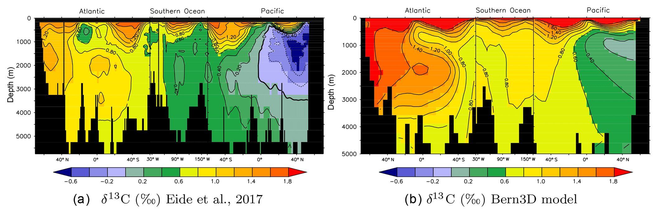
Figure 2Observed (a) versus simulated (b) preindustrial δ13CDIC distributions along a cross section through the Atlantic (25∘ W), across the Southern Ocean (58∘ S), and into the Pacific (175∘ W). (a) Data from Eide et al. (2017) based on ocean measurements and corrected for the Suess effect. (b) δ13C as modeled in the Bern3D model under preindustrial boundary conditions.
13C stocks and exchanges are modeled in the atmosphere–ocean–sediment–land biosphere system. 13C fluxes to the lithosphere associated with the burial of POC and CaCO3 and weathering input to the ocean are explicitly simulated. The burial of POC and CaCO3 results in an isotopic signature of the burial flux of around −9 ‰, intermediate between the isotopically light POC ( ‰) and the isotopically heavier CaCO3 signature (∼2.9 ‰; see Appendix A for implementation of isotopic discrimination). An isotopic perturbation in the atmosphere, e.g., through uptake of isotopically light carbon by the land biosphere, is transferred to the ocean through air–sea gas exchange and to the land by photosynthesis. Within the ocean, any perturbation is communicated between the surface ocean and the deep ocean by advection, convection, and mixing. In addition, POC and CaCO3 export fluxes from the surface ocean contribute to the burial flux.
Figure 2 shows modeled δ13C in a section through the Atlantic, Southern Ocean, and Pacific under preindustrial (1765 CE) boundary conditions with a prescribed atmospheric δ13C signature of −6.305 ‰. Compared to measured data corrected for the Suess effect (Eide et al., 2017) it is visible that modeled δ13C values are biased towards high values by a seemingly constant offset of about 0.4 ‰, while the δ13C patterns are faithfully captured by the model.
Table 1Export, burial, and deposition fluxes, as well as sediment inventories of CaCO3, opal, and particulate organic carbon (POC) as determined in the model after a preindustrial spin-up and literature estimates. The tracer input flux to the ocean resulting from weathering is set to compensate for the burial fluxes diagnosed at the end of the spin-up and kept constant in Bern3D standard simulations.
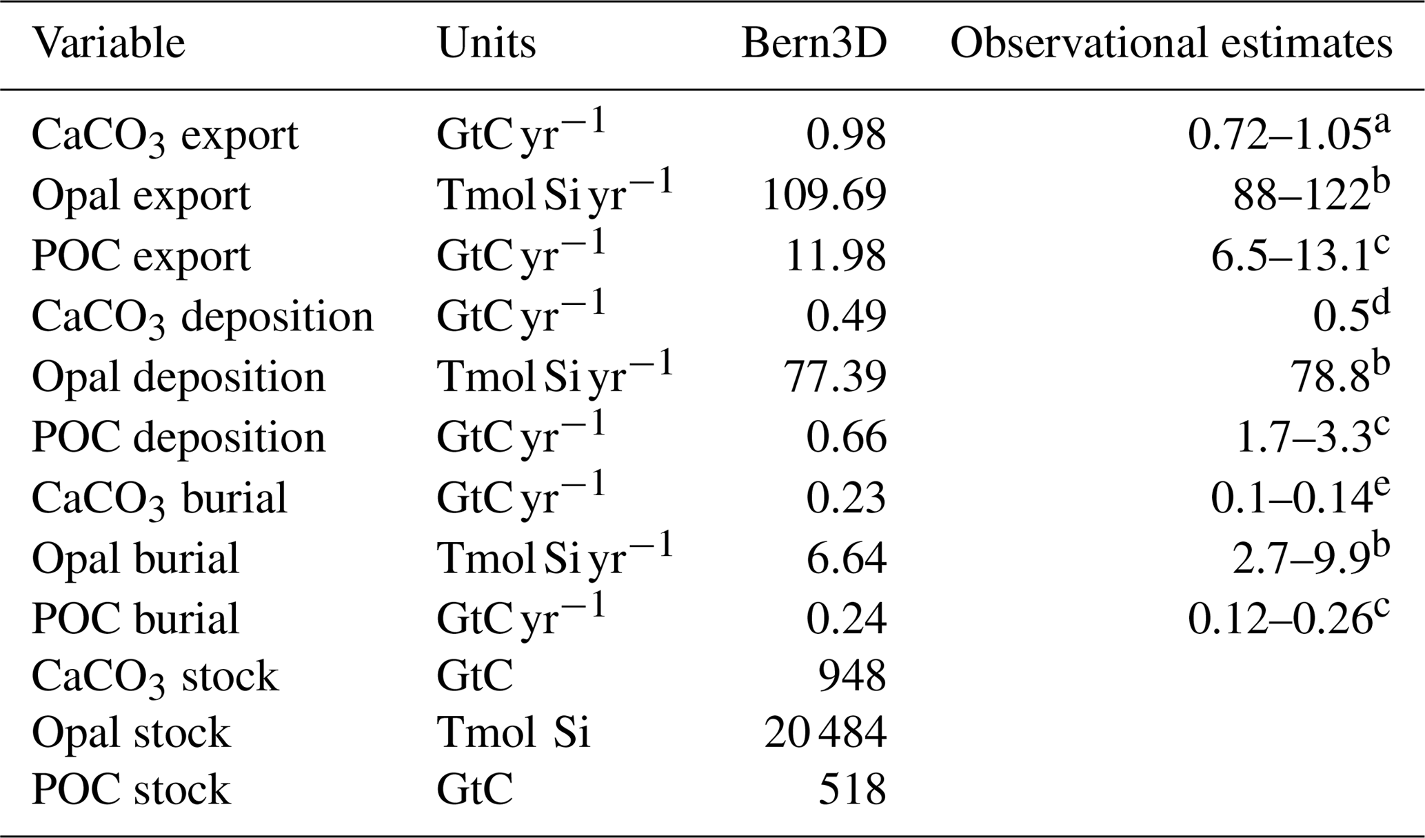
a Battaglia et al. (2016), b Tréguer and De La Rocha (2013), c Sarmiento and Gruber (2006), d Milliman and Droxler (1996), e Feely et al. (2004).
2.2 Transient LGM to PI sensitivity simulations
2.2.1 Standard transient forcings
Starting from PI steady-state conditions, the model is first run for 20 kyr under constant LGM forcing and then for an additional 20 kyr under transient forcing from the LGM to PI. Forcings (Fig. 3) include radiative forcing imposed by CO2, N2O, and CH4 (Joos and Spahni, 2008) and variations in orbital parameters (Berger, 1978). Radiative forcing of CO2 is prescribed and biogeochemistry is determined with interactive CO2. Ice sheet extent and related changes in albedo are prescribed based on benthic δ18O data (Lisiecki and Raymo, 2005) and ice sheet reconstructions (Peltier, 1994). Additionally, freshwater (FW) pulses are prescribed in the North Atlantic as detailed in Menviel et al. (2012), also accounting for the LGM to PI change in salinity of about 1 PSU. Coral reef regrowth is implemented from 14 ka onward (Vecsei and Berger, 2004) by uniformly removing the respective amount of alkalinity, carbon, and 13C from the uppermost ocean grid cells. These forcings (Fig. 3a–d) are termed standard forcings.
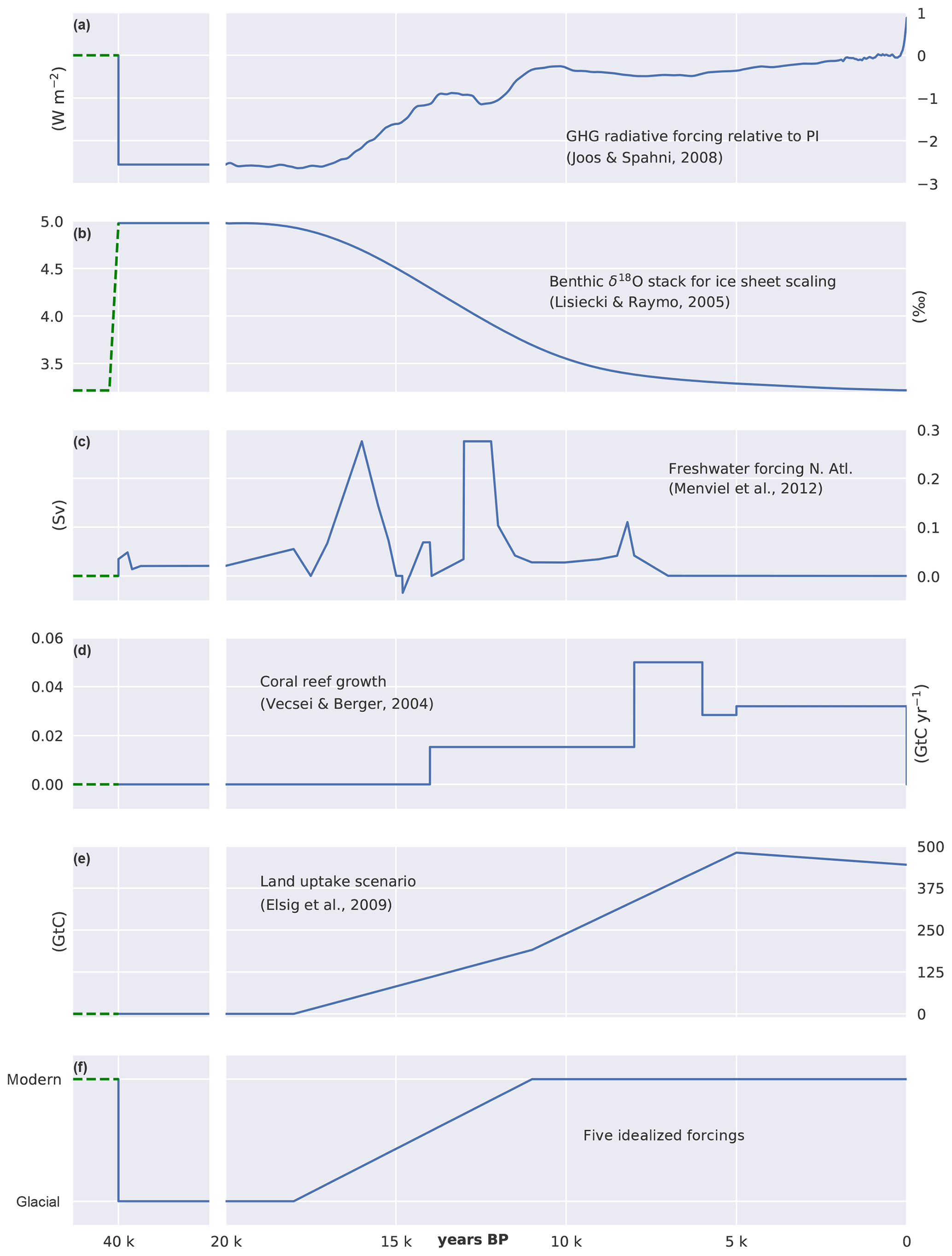
Figure 3Forcings applied for the LGM to PI simulations. (a) Radiative forcing imposed by CO2, CH4, and N2O, (b) benthic δ18O used to scale ice sheet extent, (c) freshwater forcing into the North Atlantic, and (d) coral reef regrowth as applied as standard transient forcing. (e) Prescribed evolution of land biosphere carbon uptake. Cumulative land biosphere uptake is varied over the termination across factorial simulations but kept invariant (254 GtC) over the Holocene (11–0 ka) following Elsig et al. (2009); here a scenario with a total uptake of 445 GtC is shown for illustration. (f) Idealized evolution of scaling factors as prescribed in factorial experiments to vary the remineralization profile, rain ratio, Southern Ocean wind stress and gas transfer rate, or organic weathering flux on land between LGM and PI values. The freshwater forcing in the North Atlantic is varied over 40 kyr. Dashed green lines indicate spin-up values.
2.2.2 Factorial sensitivities
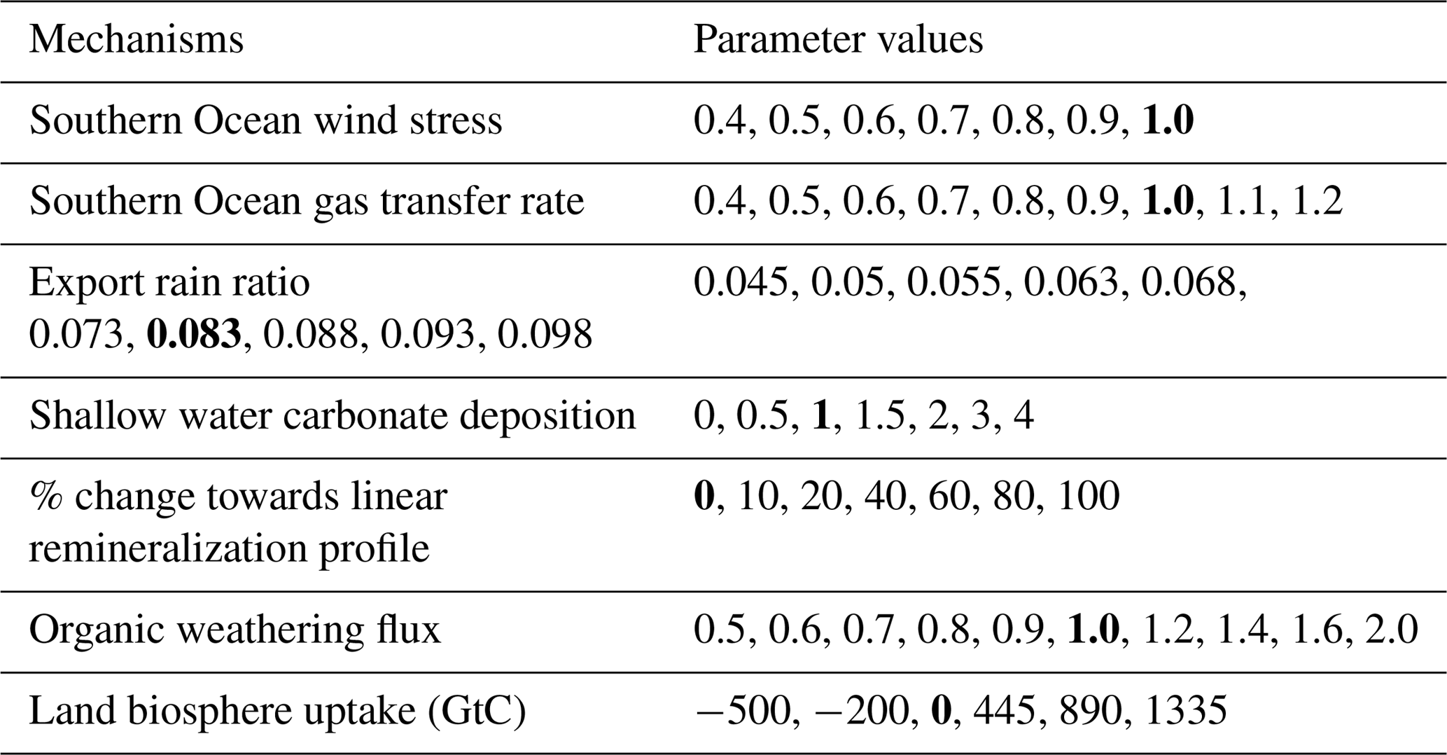
Standard transient deglacial forcings in the Bern3D model are complemented by changes in seven additional mechanisms, grouped into generic classes and introduced below (see top of Fig. 1). A set of 50 factorial experiments (Table 2), covering the same time interval as the model run with standard transient forcings, is conducted to quantify the sensitivities of the carbon cycle to changes in these seven mechanisms. The forcing history for changes in Southern Ocean wind stress, Southern Ocean gas transfer rate, the rain ratio, the remineralization profile, and the organic weathering rate are prescribed following an idealized glacial–interglacial evolution. PI values are set to LGM values at 40 ka, kept constant from 40 to 18 ka, scaled back to the PI value over the termination (18 to 11 ka), and kept constant thereafter (Fig. 3f and Table 2). The sensitivities of carbon cycle properties are obtained by subtracting the standard forcing run from the runs with complementary changes in the seven mechanisms. This also yields characteristic response relationships between different carbon cycle properties, e.g., changes in atmospheric CO2 versus changes in whole-ocean δ13C, for each process. The objective is to schematically represent the space of plausible property–property relationships for key proxies. In other words, the selected mechanisms are assumed to be representative on the global scale for the myriad of processes influencing the carbon cycle and will be outlined below.
Physical mechanisms. Changes in ocean circulation, for example in response to altered wind stress, stratification, eddy mixing, or buoyancy forcing, affect the marine carbon inventory (e.g., Adkins, 2013) by altering the cycling of organic and inorganic carbon. The Southern Ocean has been identified as an important region modulating CO2 changes, and a reduced Antarctic overturning circulation has been invoked to, at least partly, explain low glacial atmospheric CO2 (Sigman and Boyle, 2000; Sigman et al., 2010; Fischer et al., 2010; Skinner et al., 2010; Tschumi et al., 2011; Ferrari et al., 2014; Watson et al., 2015; Roberts et al., 2016; Gottschalk et al., 2016; Jaccard et al., 2016). Under standard forcing, Southern Ocean circulation changes are weak in the Bern3D model. In this study, the circulation is modified by uniformly scaling the wind stress field over the Southern Ocean ( S, south of South America) (see also Tschumi et al., 2008) to reduce deep ocean ventilation. We do not consider such large changes in wind stress to be realistic, but rather use prescribed Southern Ocean wind stress as a way to vary deep ocean ventilation in the Bern3D model. Consequently, we do not scale air–sea gas transfer rates with the changes in wind stress but vary transfer rates independently.
Proxy reconstructions suggest a larger sea-ice extent in the Southern Ocean during glacial times (Gersonde et al., 2005; Waelbroeck et al., 2009). Sea ice hinders air–sea gas exchange and thus exerts a large impact on atmospheric δ13CO2 (Lynch-Stieglitz et al., 1995). Additionally, changes in Southern Ocean winds (Kohfeld et al., 2013) may have affected glacial Southern Ocean air–sea gas transfer rates. Here, the standard air–sea gas transfer rate is scaled (Fig. 3f; Table 2) in the Southern Ocean to estimate related carbon cycle sensitivities. We note that changes in sea ice and a corresponding change in air–sea gas transfer rates are reasonably well simulated by the Bern3D model. The effect of changes in ocean temperature (Waelbroeck et al., 2009) and salinity on the solubility of CO2 is discussed elsewhere (Sigman and Boyle, 2000; Brovkin et al., 2007; Sigman et al., 2010; Menviel et al., 2012) and is part of the standard forcing.
Table 2Overview of mechanisms and parameters considered in factorial sensitivity experiments. Bold entries mark the standard parameter values. Values represent the export rain ratio at LGM, the change in remineralization profile (see text) at LGM, the scaling applied to the standard shallow water carbonate deposition history, and the land carbon uptake over the deglacial in gigatons of carbon (GtC). In the case of SO wind stress, SO gas transfer rate, and the organic weathering flux, values represent the ratio of LGM to PI forcing.
Oceanic carbonate. The partial pressure of CO2 in the ocean depends on alkalinity and processes that alter surface ocean alkalinity, thus influencing atmospheric CO2. The sedimentary burial of CaCO3 removes twice as much alkalinity as carbon from the ocean, leading to oceanic CO2 outgassing. Increased CaCO3 burial over the deglacial has been put forward as the coral reef hypothesis (Berger, 1982) to explain increases in atmospheric CO2. Vecsei and Berger (2004) reconstructed coral reef growth history and provided a lower-limit estimate of about 380 GtC for the amount of shallow water carbonate deposition over the deglacial period. Other estimates of CaCO3 deposition amount to 1200 GtC or even more (Milliman, 1993; Kleypas, 1997; Ridgwell et al., 2003). This yields a large range of possible scenarios with substantial impacts on atmospheric CO2. Here, we scale the reconstructed deposition history based on Vecsei and Berger (2004) (Fig. 3d) by applying a constant scaling to vary CaCO3 deposition within the published range.
Potential changes in the rain ratio (CaCO3 : Corg) affect both alkalinity and CO2 (e.g., Berger and Keir, 2013; Archer and Maier-Reimer, 1994; Sigman et al., 1998; Archer et al., 2000; Matsumoto et al., 2002; Tschumi et al., 2011). An increase in the export of CaCO3 relative to Corg from surface waters has similar consequences for CO2 as shallow water carbonate deposition (Sigman and Boyle, 2000). There is a lack of estimates on how the rain ratio has varied in the past. Here, we vary the global rain ratio for LGM conditions (see also Appendix A; Fig. 3f; Table 2) between 0.045 and 0.098, while the rain ratio is 0.083 in the standard setup and for PI conditions.
Oceanic organic matter. There is a broad range of mechanisms, in addition to circulation changes, that affect the cycling of organic matter within the ocean, the whole-ocean nutrient inventories, and thereby surface ocean nutrient and DIC concentrations as well as atmospheric CO2. Several studies have suggested changes in the remineralization length scale of organic carbon due to colder ocean temperatures (see, e.g., Matsumoto, 2007; Menviel et al., 2012; Roth et al., 2014). A deeper remineralization of organic matter leads to the removal of nutrients and DIC from the shallow subsurface ocean and, via ocean–sediment interactions, to globally reduced nutrient and increased alkalinity inventories (Menviel et al., 2012; Roth et al., 2014), resulting in a decrease in atmospheric CO2 (Matsumoto, 2007; Menviel et al., 2012). Weathering–burial feedbacks lead to an amplification of changes in atmospheric and oceanic δ13C as shown by Tschumi et al. (2011) and Roth et al. (2014). Here, the remineralization profile in the upper 2 km is varied between the standard Martin curve (Eq. A1 in Appendix) and a linear profile (75 to 2000 m). The modification in the remineralization profile of particulate organic matter is different than those applied by Menviel et al. (2012) and Roth et al. (2014) in simulations with the Bern3D model. Here, only the remineralization profile in the upper 2000 m is changed, and, in contrast to these earlier studies, it is assumed that the fraction of exported particles that reach the sediments below 2000 m is not altered. The implicit assumption is that cooler temperatures at the LGM only significantly affect the dissolution of relatively small or labile particles in the upper ocean, while large or refractory particles sink fast enough to reach ocean sediments both under LGM and PI conditions.
Oceanic organic carbon and nutrient inventories are further affected by changes in the weathering flux compensating for the burial of organic matter (Cartapanis et al., 2016, 2018). A negative balance between the riverine input of PO4, DIC, DI13C, and Alk, originally buried as organic material, and sedimentary burial of particulate organic matter leads to a transient decrease in atmospheric CO2 and also affects atmospheric and marine δ13C. The weathering flux to the ocean (Table 1) is kept constant in the standard setup of the Bern3D (see also Appendix A) but might have varied with changes in climate and CO2. To account for this possibility, we varied the input of PO4, DIC, DI13C, and Alk that compensates for the burial of particulate organic material in the sediment in factorial experiments (Fig. 3f; Table 2). This variation in the input will be referred to as changes in the organic weathering flux.
Another widely discussed mechanism relates to iron fertilization in the Southern Ocean (Martin, 1990; Archer et al., 2000; Sigman and Boyle, 2000; Parekh et al., 2008; Sigman et al., 2010; Fischer et al., 2010; Martinez-Garcia et al., 2014). Iron fertilization leads to changes in the cycling of marine organic material and to related changes in the whole-ocean inventory of δ13CDIC and other variables. These changes are broadly similar to the changes caused by altering the organic matter remineralization depth or the weathering input flux and implicitly included in the Monte Carlo simulations. Similarly, other processes, such as changes in the ratio of nutrient to carbon uptake by marine organisms (Heinze et al., 2016) or changes in the association of POC with ballast minerals (Armstrong et al., 2002), may have affected the efficiency of the marine biological cycle in reducing carbon in the surface ocean and the atmosphere.
Land biosphere carbon inventory. Changes in land biosphere carbon stock are prescribed following the evolution illustrated in Fig. 3e. We assume that the change in land carbon stock over the Holocene is well constrained and amounts to an uptake of 290 GtC at 11–5 ka and a release of 36 GtC thereafter (Elsig et al., 2009). Scenarios with different cumulative land carbon change imply a corresponding uptake or release of terrestrial carbon during the last glacial termination (18–11 ka). The δ13C signature of terrestrial carbon is set to −24 ‰.
2.2.3 Data constraints for deglacial carbon and carbon isotope changes
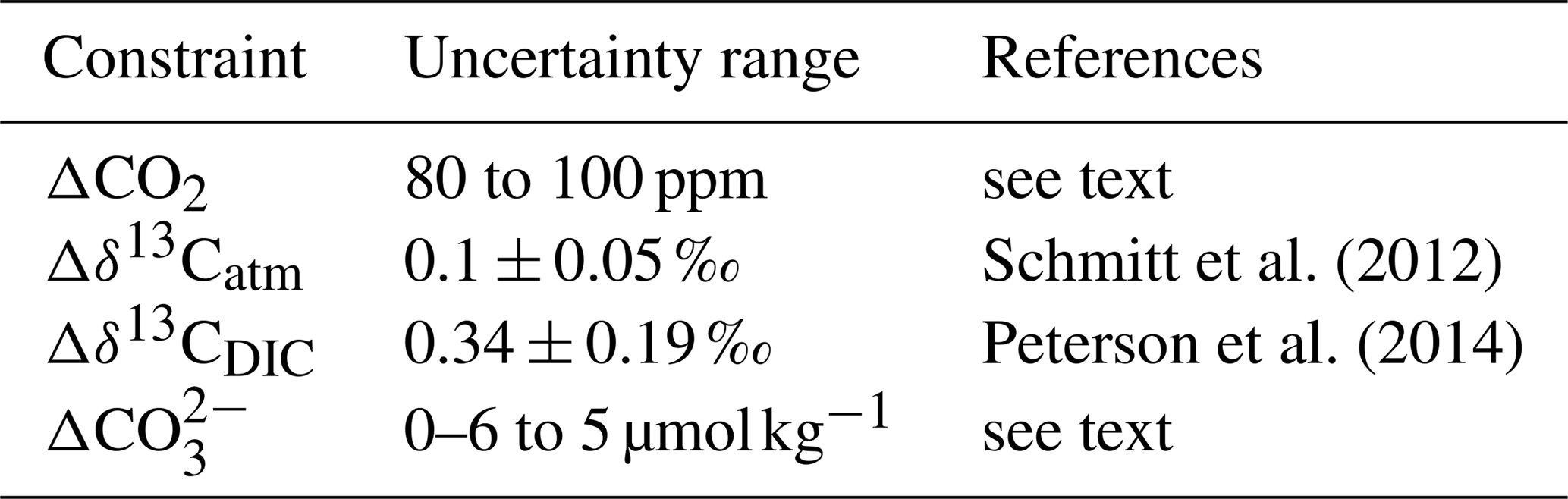
We consider four globally relevant observational constraints (Table 3) to estimate the PI–LGM change in the land biosphere carbon inventory, Δland. These are the PI–LGM difference (Δ) in (i) atmospheric CO2 (ΔCO2), (ii) atmospheric δ13C(CO2) (Δδ13Catm), (iii) mean ocean δ13C(DIC) (Δδ13CDIC), and (iv) deep (equatorial) Pacific carbonate ion concentration () (Table 3). The carbon isotope constraints are directly relevant for the isotopic mass balance used to infer Δland. The carbonate ion concentration difference constrains changes in the ocean's alkalinity budget, and the change in atmospheric CO2 constrains the integrated effect of deglacial carbon cycle changes. We allow for a relatively wide uncertainty range of 20 ppm for ΔCO2, which is admittedly wider than the proxy uncertainty, to avoid an overfitting of model outputs. The Δδ13Catm range for the constraint is 0.1±0.05 ‰ and based on ice core measurements (Schmitt et al., 2012). Peterson et al. (2014) compiled 480 benthic foraminiferal records and report a whole-ocean PI minus LGM change in δ13CDIC of 0.34±0.19 ‰, and we use their range (0.15 ‰ to 0.53 ‰) as a constraint. Proxy reconstructions of based on measured B∕Ca ratios in foraminifera show little change from LGM to PI in the equatorial deep Pacific (Yu et al., 2013). Based on a different approach, Qin et al. (2017) also conclude on negligible change in in the western tropical Pacific across the last glacial termination. In a recent study, Luo et al. (2018) report, based on CaCO3 reconstructions in the South China Sea, that carbonate ion concentrations in the mid-depth Pacific hardly changed from LGM to PI. All these studies point to a small change in , providing a further constraint on deglacial simulations. However, the uncertainty in these reconstructions is of the same order as the change itself. The target range for is chosen here from −6 to 5 µmol kg−1.
Schmitt et al. (2012)Peterson et al. (2014)Table 3Overview of the four proxy-based constraints representing change (Δ) between PI minus LGM. LGM refers to the period 20 to 19 ka for the ice core and to the period 23 to 19 ka for the ocean sediment data. Similarly, PI refers to 500 to 200 BP for the ice core data and 6000 to 200 BP and 8 to 6 ka for marine δ13C and , respectively. The assumed uncertainty range in ΔCO2 is considered to be wider than the uncertainty from the ice core data. This is to avoid overfitting and taking into account uncertainties in the emulator introduced in Sect. 2.2.4.
2.2.4 Emulator and Monte Carlo setup
Sensitivities of the four target proxies (ΔCO2, Δδ13Catm, Δδ13CDIC, and ) to changes in the selected seven forcings are computed based on 50 factorial experiments. For each forcing, i, and related parameter change, Δpi (Table 2), the corresponding sensitivity, i.e., the change in target per unit change in parameter, is computed. These discrete sensitivities are fitted linearly or quadratically for each target, T, and forcing to get a continuous function for the sensitivity, (Δpi). These sensitivity functions are used to build a simple representation to compute changes in target variables for a combination of changes in parameters:
In order to evaluate the assumed linear additivity of the seven mechanisms, a 60-member ensemble of parameter combinations is calculated both with the Bern3D model and Eq. (1) (Fig. 1). The seven parameters are sampled uniformly using Latin hypercube sampling (LHS; McKay et al., 1979). The results from the Bern3D model and Eq. (1) are regressed against each other for each target variable (Fig. C1). The corresponding linear fit is used to account for nonadditive behavior when combining forcings. This then yields the following emulator:
where aT is the offset and bT the slope of the respective linear fit as given in Appendix Fig. C1. The root mean square deviation between the emulator (Eq. 2) and the Bern3D model is 8.8 ppm for ΔCO2, 0.06 ‰ for Δδ13Catm, 0.02 ‰ for Δδ13CDIC, and 4 µmol kg−1 for . The seven parameters of the LGM to PI sensitivity experiments are sampled uniformly by drawing random samples over their employed ranges (Table 2) to generate a 500 000-member Monte Carlo ensemble. The above emulator is used for each of these members to estimate the corresponding changes in the four targets. Members that yield changes in the targets that lie outside the defined ranges (Table 3) are excluded from the analysis; all remaining members are used to calculate median and confidence ranges in Δland and other variables of interest.
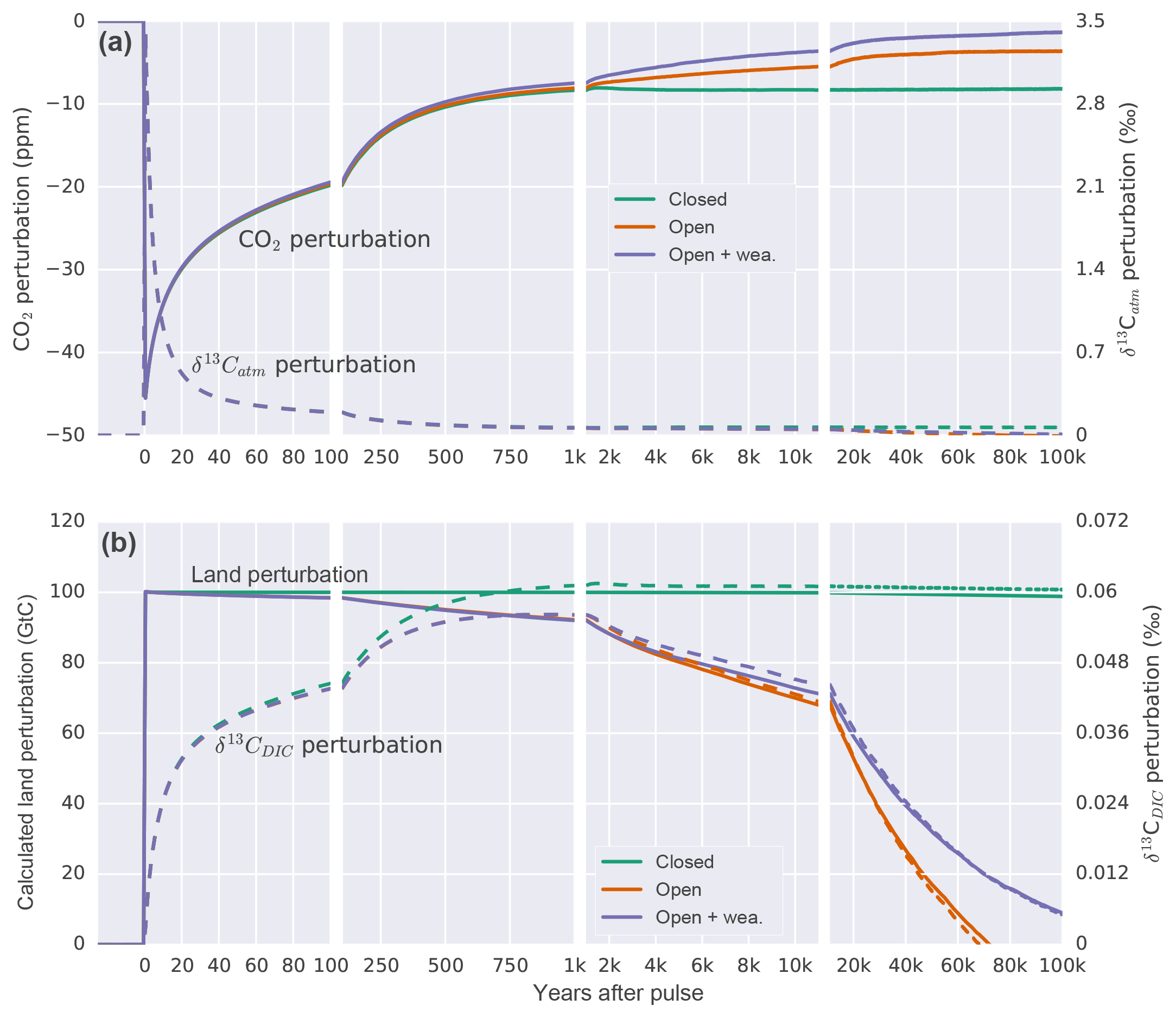
Figure 4Temporal evolution of the perturbation in (a) atmospheric CO2 and δ13Catm. (b) The calculated perturbation in terrestrial carbon storage following Eqs. (A2) and (A3) and δ13CDIC anomalies for a pulse uptake of 100 GtC by the land in a closed (green), open (orange), and open system with enabled weathering feedback (purple). Solid lines refer to left and dashed lines to right y axis in both panels.
3.1 Pulse experiments
We start by investigating how atmospheric CO2 and δ13C signatures evolve in response to carbon uptake by the land biosphere when all other forcings remain unchanged. To this end, 100 GtC of light carbon ( ‰) is instantaneously (in the first time step of the year) removed from the model atmosphere to test the Bern3D response for different model setups (see Appendix A). This yields the Green's functions (or impulse response functions) for carbon and 13C shown in Fig. 4.
First, we apply the pulse to a closed system, which includes only the atmosphere, ocean, and land biosphere components. The removal of 100 Gt of light carbon from the atmosphere results in an initial decline in atmospheric CO2, followed by a typical impulse–response recovery (e.g., Maier-Reimer and Hasselmann, 1987; Siegenthaler and Joos, 1992). Atmospheric CO2 recovers as the ocean starts to outgass CO2 (Fig. 4). In a closed system, atmospheric CO2 reaches a new equilibrium after about 2 kyr, at 8 ppm below the initial steady state. As light carbon is removed, the remaining carbon in the ocean and atmosphere becomes relatively enriched in 13C. Initially, the δ13Catm perturbation is removed much faster than the atmospheric CO2 perturbation as exchange with the ocean and land biosphere dilutes the imposed isotopic perturbation (Fig. 4a; Joos and Bruno, 1996). The oceanic δ13C increases and equilibrates after about 2 kyr. The difference in the response of CO2 and δ13C is related to their different properties. CO2 represents a concentration, whereas δ13C stands for the isotopic ratio of 13C to 12C. The capacity of the ocean to remove an atmospheric perturbation in CO2, and equally in 12CO2 and 13CO2, is limited by the acid–base carbonate chemistry described by Revelle and Suess (1957). In contrast, the removal of a perturbation in the isotopic ratio 13CO2∕12CO2 is hardly affected by this chemical buffering; the buffering affects 13CO2 in the nominator and 12CO2 in the denominator about equally, leading to a near cancellation of its effect on the ratio. The resulting change for the new equilibrium in δ13C amounts to 0.066 ‰ for the atmosphere, 0.060 ‰ for the ocean, and 0.065 ‰ for the four-box land biosphere. The mass balance between ocean, land, and atmosphere is maintained such that the inferred land perturbation (calculated using Eqs. A2 and A3) corresponds to the prescribed removal of 100 GtC (Fig. 4b).
In the second open system experiment, marine sediments are included. The evolution of atmospheric CO2 (see Archer et al., 1998) is similar to the closed system except that CaCO3 compensation leads to a further recovery of atmospheric CO2 until equilibrium is approached with an e-folding timescale of about 14 000 years. CO2 equilibrates at around 3.5 ppm below the initial steady state. For the first thousand years, the evolution of δ13C in the atmosphere and ocean is comparable to the closed system experiment but differs thereafter.
The novel and most important finding from the pulse experiment is that the δ13C perturbation in the ocean–atmosphere–land biosphere system is increasingly and eventually completely removed by open system processes. Figure 4b shows the δ13CDIC perturbation to decrease on a multi-millennial timescale in contrast to the closed system assumption (dashed lines in Fig. 4b). In other words, benthic foraminifera record a much smaller perturbation in seawater δ13C than expected from closed system modeling. The resulting difference in the δ13CDIC perturbation between the open and closed system causes an erroneous mass balance inference for the terrestrial biosphere when applying conventional closed system equations (Eq. A2 and A3). On a timescale of 10 kyr, underestimation of the terrestrial carbon inventory change amounts to 30 %. The error increases as time evolves.
In detail, the difference between the open and closed system pulse responses is explained as follows. The 13C budget in the open system changes due to imbalances between input and burial fluxes of POC and CaCO3 and due to changes in the δ13C signatures of the respective fluxes. The uptake of isotopically light land carbon from the atmosphere leads to an increase in the δ13C signature of surface waters and through that in the δ13C signatures of exported and eventually buried POC and CaCO3. The mean δ13C signature of the burial flux amounts to −8.7 ‰ (δ13C: 2.9 ‰) and Corg (δ13CPOC: −20.2 ‰) for the first 10 kyr compared to −9.1 ‰ for the weathering input. This difference tends to mitigate the δ13CDIC perturbation. Further, carbon–climate feedbacks cause changes in temperature and ocean circulation, which affect the export of POC and CaCO3. Burial fluxes of POC further depend on O2 concentrations and burial fluxes of CaCO3 on concentrations that evolve over the course of the simulation. As a result, the cumulative sedimentation–weathering imbalance amounts to a removal of 48.5 GtC during the first 10 kyr. The contribution to differences in the carbon isotopic budget relative to the closed system is dominated by changes in POC cycling and its associated δ13C signature, while changes in the CaCO3 cycle play a smaller but non-negligible role. Overall, 13C is lost from the atmosphere–ocean system, and δ13CDIC is decreasing.
In the third pulse experiment, changes in global mean air temperature and atmospheric CO2 concentration affect weathering fluxes of CaCO3 and CaSiO3 following Colbourn et al. (2013). The implemented feedbacks cause a reduction in modeled weathering fluxes in response to decreased atmospheric CO2 and temperature over the course of the experiment. Decreased weathering fluxes of CaCO3 and CaSiO3 lead to a decline in alkalinity supplied to the ocean, resulting in a net transfer of carbon to the atmosphere. This further reduces the initial CO2 perturbation (Fig. 4a). The mean δ13C value related to weathering is −9.1 ‰, thereby leading to a slightly higher δ13CDIC perturbation at 10 kyr compared to the open system experiment with fixed weathering fluxes. The error related to the calculated land perturbation is comparable on a 10 kyr time horizon and increases less as time progresses further compared to the open system setup with fixed weathering.
The pulse responses make it clear that open system processes such as sediment interactions, burial, and weathering affect the carbon and δ13C budgets on deglacial timescales. Taken at face value, the results suggest that the classical δ13C-based estimates of Δland are substantially biased low because of the neglect of open system processes. However, uptake by land carbon is the only forcing in these idealized pulse simulations, whereas climate and biogeochemical cycles underwent a massive reorganization over the glacial–interglacial transition. This reorganization affected open system processes and the 13C budget in addition to carbon uptake by the land biosphere. In the next section, we estimate Δland by taking into account deglacial processes.
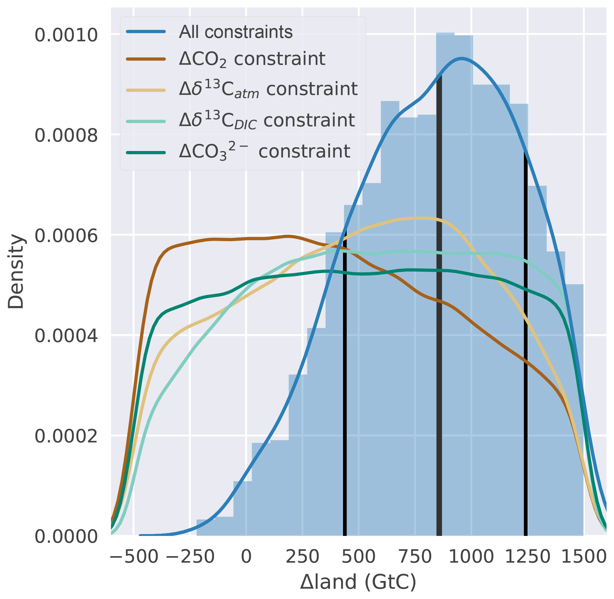
Figure 5Histogram (blue bars, normalized) and kernel density estimate (blue line) of Δland wherein parameter combinations fulfill all four data-based constraints. The thick vertical black line indicates the median Δland of ∼850 GtC, and thin black lines show the ±1σ range. The remaining four lines show kernel density estimates of Δland when considering one data-based constraint at a time.
3.2 Ensemble approach to constrain Δland
We represent the deglacial reorganization of the ocean in the standard model setup, complemented by the seven deglacial carbon cycle mechanisms and constrained by the four observational targets within an open system model framework. Applying the Bern3D emulator (Eq. 2) to our 500 000-member parameter ensemble, we find that the prior range in Δland, ranging from −500 to 1500 GtC, is constrained to ∼450 to ∼1250 GtC (±1σ range; see Fig. 5). The constrained median amounts to ∼850 GtC, and almost no ensemble members that fulfill all four observational constraints are found for negative Δland values. The constrained ensemble thus clearly suggests a positive Δland.
Next, we show that it is not sufficient to use Δδ13CDIC, or any other target, in isolation to constrain Δland. The probability distribution of Δland covers the whole range of sampled values almost uniformly (Fig. 5) when applying only one out of the four targets. Considering either Δδ13CDIC or Δδ13Catm together with ΔCO2 as constraints moves the Δland distribution towards the multi-proxy-based distribution (blue line in Fig. 5; not shown). We conclude that the incorporation of multiple constraints is essential to narrow uncertainties in Δland.
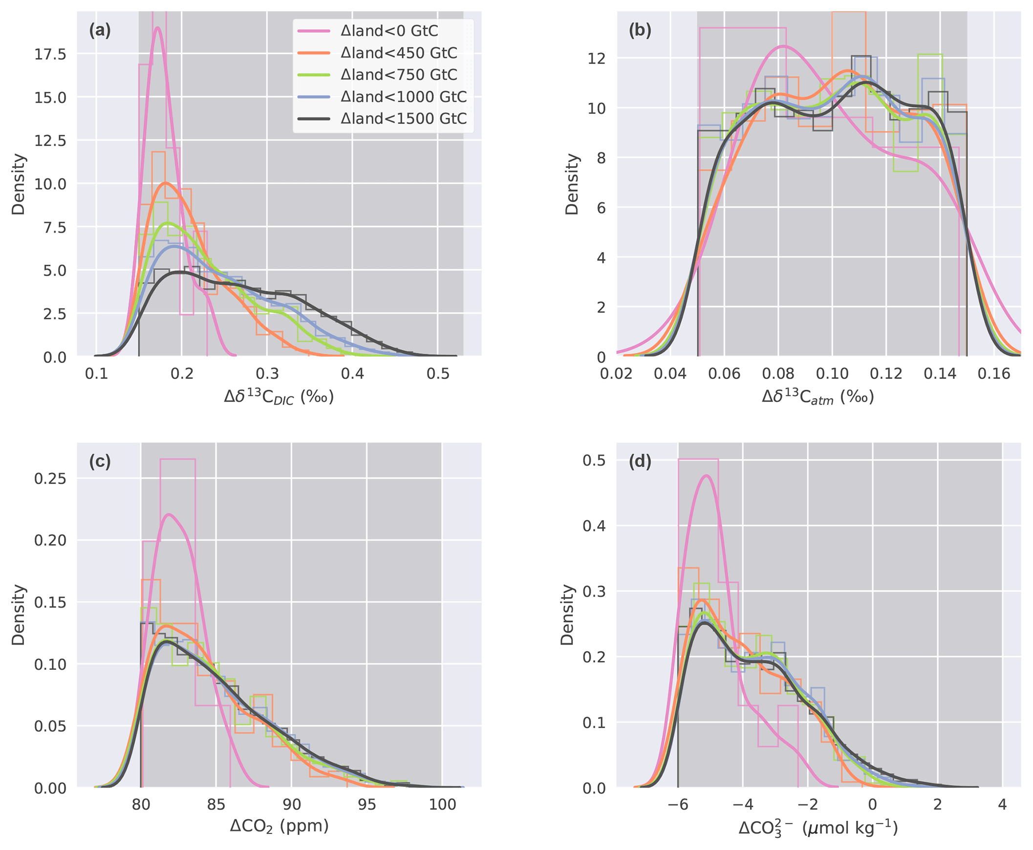
Figure 6Histogram (thin lines, normalized) and kernel density estimate (thick lines) of (a) Δδ13CDIC, (b) Δδ13Catm, (c) ΔCO2, and (d) values for parameter combinations calculated with the emulator that fulfill the observational constraints. Different colors in all four panels correspond to subsamples divided along Δland values that are smaller than 1500, 1000, 750, 450, and 0 GtC. Darker grey shading indicates the range of the respective observational constraint.
Our unconstrained ensemble yields a very large spread in the four target variables. Δδ13CDIC ranges from −0.77 ‰ to 1.25 ‰, Δδ13Catm from −0.9 ‰ to 1.32 ‰, ΔCO2 from −107 to 181 ppm, and from −49 to 42 µmol kg−1. Within the optimization procedure, we specify that only defined, observation-based ranges of these target variables are allowed (Sect. 2.2.3) and that all four of these constraints have to be met at the same time. This yields specific distributions of the target variables within our constrained ensemble (Fig. 6, black lines). The distribution of Δδ13Catm values, for instance, is almost uniform within the defined observational range (Fig. 6b), while ΔCO2, , and Δδ13CDIC values cluster towards the lower end of the specified target ranges (Fig. 6c, d, a). This is a result of the underlying carbon cycle–climate processes as tested within Bern3D. For example, it remains difficult to model a PI–LGM ΔCO2 of ∼90 ppm under the constraint of meeting the other three observational targets. Most ensemble members represent a ΔCO2 of ∼82 ppm (Fig. 6c). Higher ΔCO2 values are present in the unconstrained ensemble but are generally associated with even more negative (not shown), which is outside the defined target range for .
We stratify the results by Δland and define four sets in which Δland is allowed to be maximally 1000, 750, 450, and smaller than 0 GtC (Fig. 6, blue, green, orange, and magenta lines). Only one target variable, Δδ13CDIC, is sensitive to this restriction within the constrained ensemble and positive Δland. The distributions of Δδ13Catm, ΔCO2, and are almost identical for all subsets of Δland with the exception of Δland, which is smaller than 0 GtC. Hence, these three targets do not discriminate per se between smaller and larger estimates of positive Δland. In contrast, restricting Δland to smaller values shifts the realized Δδ13CDIC towards lower values, and the mean of the constrained distribution shifts away from the mean observational estimate of 0.34 ‰ (Fig. 6a). For example, Δδ13CDIC is always below 0.35 ‰ for Δland, below 450 GtC, and always below 0.23 ‰ for negative Δland estimates. Thus, not only do very few process combinations yield a negative Δland in our 500 000-member ensemble (Fig. 5), but these solutions are also biased low in Δδ13CDIC. Further, solutions with negative Δland also yield ΔCO2 and values at the very low end of the observational constraints (Fig. 6b, c). Taken together, our framework strongly suggests that the land biosphere sequestered carbon over the deglaciation and that the sequestered amount is likely larger than 450 GtC.
3.3 Carbon and δ13C changes in LGM to PI sensitivity simulations
This section is intended for readers interested in a more detailed quantification of deglacial carbon cycle mechanisms. We recall that the model is initialized with a spin-up for PI conditions and simulations started 40 ka under LGM forcing (Fig. 3). Forcing the model from PI into an LGM state by applying standard forcings leads to a shoaling and slight slowdown of the Atlantic meridional overturning circulation (AMOC) of about 4.4 Sv (PI steady state: 18 Sv) and a global cooling of the ocean and the atmosphere of about 1.4 and 3 ∘C over the glacial, respectively. New production of organic matter decreases from 11.98 GtC yr−1 to a mean value over the glacial of 11.25 GtC yr−1. The oceanic carbon inventory increases at the expense of the atmosphere, yielding a higher concentration during the glacial. Turning to the deglaciation, CO2 increases by 27.8 ppm from LGM to PI, while δ13Catm and δ13CDIC show little change between LGM and PI (Fig. 7). By applying the standard transient forcings alone, neither the Δδ13C constraints in the atmosphere and ocean nor the ΔCO2 constraint is met, calling for the consideration of additional processes.
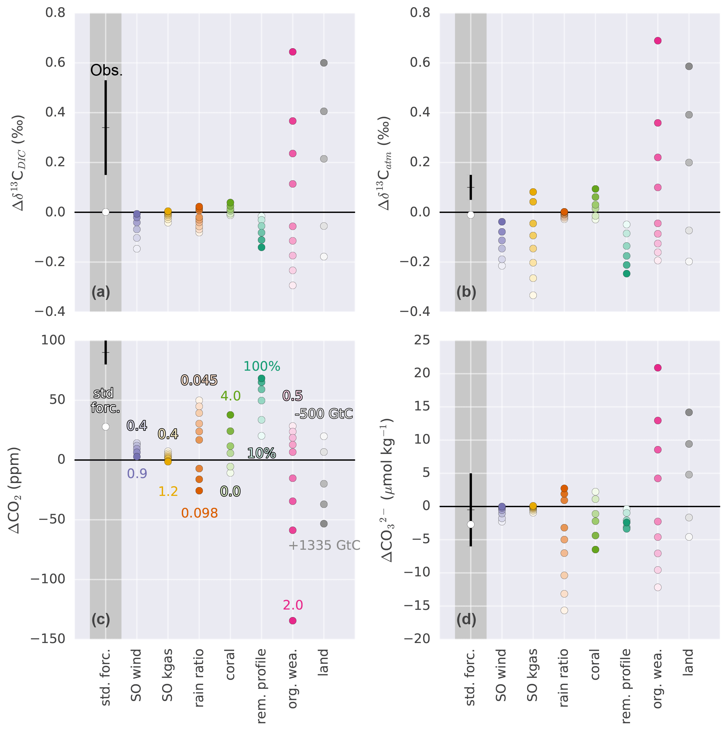
Figure 7Sensitivity of (a) Δδ13CDIC, (b) Δδ13Catm, (c) ΔCO2, and (d) to changes in Southern Ocean wind stress (SO wind), Southern Ocean gas transfer rate (SO kgas), export rain ratio, shallow water carbonate deposition (coral), remineralization profile (rem. profile), organic weathering flux (org. wea.), and land carbon uptake (land). Sensitivities are shown relative to the standard forcings (white dots). Values in panel (c) correspond to the entries in Table 2. Black crosses with error bars show estimates based on measurements (ΔCO2: Petit et al., 1999; Monnin et al., 2001; Siegenthaler et al., 2005; Lüthi et al., 2008; Köhler et al., 2017; Δδ13Catm: Schmitt et al., 2012; : Yu et al., 2013; Qin et al., 2017; Luo et al., 2018; Δδ13CDIC: Peterson et al., 2014). Dots in dark grey shading show absolute and in light grey shading relative (to standard forcings) values. Δ indicates the PI–LGM difference.
3.3.1 Sensitivity of carbon cycle processes to changes in additional deglacial processes
The mean δ13C signature of the ocean–atmosphere system changes in response to potential deglacial processes (Fig. 7a–b). For simplicity, we focus on the change in mean ocean δ13CDIC (Fig. 7a) as the ocean holds about 20 times more carbon than the atmosphere and interactive land biosphere together. The factorial simulations reveal a Δδ13CDIC (PI–LGM) between −0.3 ‰ and more than 0.6 ‰ when halving or doubling the weathering flux of organic material, respectively. Prescribed changes in Southern Ocean (SO) wind stress inducing changes in ocean circulation, the organic matter remineralization profile, and in the rain ratio lead to a change in the ocean signature of about −0.2 ‰, while changes in the SO air–sea gas transfer rate and in coral reef growth have a small influence on Δδ13CDIC. The influence of these mechanisms on δ13CDIC cannot be ignored when estimating Δland based on reconstructed changes in δ13C.
Reconstructions of the change in δ13C in the atmosphere and ocean differ in magnitude. The change in the atmosphere (0.1±0.05 ‰) is about one-third of the oceanic change (0.34±0.19 ‰). Changes in the organic weathering flux and terrestrial carbon storage affect Δδ13CDIC and Δδ13Catm in an identical way. Changes in SO wind stress, rain ratio, coral reef growth, and the remineralization of organic material have a similar influence on the two isotope variables. In contrast, changes in the SO air–sea gas transfer rate alter Δδ13Catm, while hardly changing Δδ13CDIC. The strong sensitivity of δ13Catm to changes in SO gas transfer rate is due to the large disequilibrium between the atmosphere and surface ocean. This makes this process, in addition to temperature-driven changes in fractionation, potentially important in setting atmospheric δ13C independently from mean ocean δ13CDIC change (see also Fig. C2b).
Considering ΔCO2 and , the changes in investigated mechanisms significantly influence atmospheric CO2 and deep Pacific carbonate ion concentration (with the exception of air–sea gas transfer rate). A general relationship becomes apparent. A positive change in ΔCO2 is always accompanied by a negative change in and vice versa (Fig. 7c–d). Thus, the explanation for the observed deglacial increase in CO2 of ∼90 ppm requires a deglacial decrease in deep Pacific carbonate ion concentration (Fig. 6d), at least in our model and considering the mechanisms implemented in the standard and factorial simulations. Changes in alkalinity and DIC (PI–LGM) for the standard forcing amount to about 500 Gt and 365 GtC, respectively. In the case of rain ratio, coral reef growth, and changes in the remineralization profile, changes in alkalinity and DIC are largest and occur close to a 2:1 ratio. Changes in land carbon uptake remove carbon from the system, leading to changes in alkalinity via CaCO3 compensation, whereas in the case of the organic weathering flux, not only carbon is added and/or removed from the system but also nutrients and alkalinity, following Redfield ratios (see Appendix A). Changes in alkalinity and DIC resulting from changes in Southern Ocean wind stress and gas transfer rate are small.

Figure 8ΔCO2 for defined sensitivity experiments plotted against (a) Δδ13Catm, (b) Δδ13CDIC, (c) , and (d) Δδ13Catm vs. Δδ13CDIC. Black crosses indicate results with standard forcings alone, and dark grey shading shows ranges for data-based constraints (ΔCO2: Petit et al., 1999; Monnin et al., 2001; Siegenthaler et al., 2005; Lüthi et al., 2008; Köhler et al., 2017; Δδ13Catm: Schmitt et al., 2012; : Yu et al., 2013; Qin et al., 2017; Luo et al., 2018; Δδ13CDIC: Peterson et al., 2014). For the direction of change in the forcings see Fig. 7. Note that in (a) changes in Δland that yield a positive ΔCO2 are overlaid by the organic weathering flux line.
3.3.2 Response relationships between different carbon cycle properties
The results for the target variables are plotted against each other to gain further insight into the relative importance of the different mechanisms to meet the observational constraints (Fig. 8). This yields a characteristic slope for each target pair and mechanism. For example, this slope is negative and equates to about −90 ppm ‰−1 for the pair ΔCO2 and Δδ13CDIC and the mechanism of land carbon storage (grey line in Fig. 8a). Roughly similar slopes are found for variations of the organic weathering flux, SO wind stress, and SO air–sea gas transfer rate. Figure 8a reveals that variations in these four processes cannot prompt the model results to agree with these two observational constraints. The slopes are too small in magnitude and either ΔCO2 or Δδ13CDIC remains outside the observational range. The four processes are effective in varying Δδ13CDIC but relatively ineffective in varying ΔCO2. Processes that have a much larger impact on ΔCO2 than on Δδ13CDIC are related to the CaCO3 cycle (coral reef growth and rain ratio) and changes in the upper ocean remineralization of particulate organic matter. This implies that variations in Δland, organic weathering, and ocean circulation (SO wind) are required to meet the Δδ13CDIC target, while variations in coral reef regrowth, rain ratio, and upper ocean remineralization depth are necessary to meet the ΔCO2 target. Indeed, the median changes for the parameters in the observationally constrained ensemble (Fig. C2) imply a deeper remineralization of organic matter and a reduced rain ratio at LGM than PI and a 3 to 4 times higher amount of CaCO3 deposition during coral reef regrowth than applied in the standard run. These, together with a reduced SO wind stress at the LGM, all contribute to a deglacial increase in CO2. The associated decrease in Δδ13CDIC from these changes is in most Monte Carlo realizations more than compensated for by a deglacial increase in land carbon inventory and in many realizations by an increased glacial organic weathering flux (Figs. C2, 8f–g). In general, the smaller the change in Δland, the larger the increase required in the glacial flux of organic weathering.
Slopes for the target pair Δδ13Catm−ΔCO2 resemble the Δδ13CDIC−ΔCO2 pair (Fig. 8a–b). Variations in SO air–sea gas transfer rate, SO wind stress, Δland, and organic weathering flux show relatively high sensitivity for Δδ13Catm and low sensitivity for ΔCO2, whereas coral reef regrowth, rain ratio, and upper ocean remineralization changes exert a large impact on ΔCO2 and affect Δδ13Catm little (Fig. 8b). In contrast to the Δδ13CDIC−ΔCO2 target pair (Fig. 8a), the slopes for the Δδ13Catm−ΔCO2 pair do not fall on roughly two characteristic slopes but vary across processes (Fig. 8b).
The clear relationship between oceanic alkalinity and oceanic carbon uptake (Fig. 7c–d) is also visible in Fig. 8c. Higher alkalinity during the glacial (negative ) generally results in a larger drawdown of atmospheric CO2 (positive ΔCO2). An interesting exception is that a modest deepening of the remineralization of organic matter in the upper ocean leads to large changes in atmospheric CO2, while at the same time hardly changing deep Pacific , making it a potentially important process to fulfill the ΔCO2 target without shifting away from the observationally constrained range (Fig. 8c). Accordingly, the remineralization depth of organic matter is deeper at the LGM than PI in all Monte Carlo realizations (Fig. C2e).
Next, we consider the Δδ13C target pair (Fig. 8d). The difficulty in simultaneously fulfilling the atmospheric and oceanic δ13C constraints with a negative Δland is becoming obvious. With negative Δland, Δδ13Catm and Δδ13CDIC are both moved towards negative values relative to standard forcings. Therefore, the isotopic constraints could only be fulfilled with an increased glacial organic weathering flux such that Δδ13Catm and Δδ13CDIC are both moved towards positive values relative to the standard forcings (Fig. 8d). Considering the ΔCO2 and constraints (Fig. 8c) implies that negative Δland can only be offset by increased glacial organic weathering or rain ratio. However, reaching a ΔCO2 of 80–100 ppm remains difficult for negative Δland when combining information from all panels of Fig. 8. This explains why only very few solutions with negative Δland and no solutions with Δland smaller than −220 GtC are found in the Monte Carlo simulations (Sect. 3.2).
3.3.3 Sensitivity of the spatial distribution of Δδ13CDIC to changes in deglacial processes
In this section, we describe the spatial distribution of changes in Δδ13CDIC. The reference run with standard LGM forcings (Fig. 9a) shows substantial spatial changes in Δδ13CDIC from internal reorganization linked to ocean circulation changes. Reduced glacial ocean ventilation as evidenced in changes in ideal age leads to the accumulation of light carbon from marine export productivity in the ocean interior. Circulation changes hence explain the variability in the spatial pattern of Δδ13CDIC in Fig. 9a. In particular, the deepening and strengthening of the AMOC during the deglaciation lead to positive Δδ13CDIC changes in the deep Atlantic and to negative Δδ13CDIC changes in the upper Atlantic, consistent with proxy reconstructions.
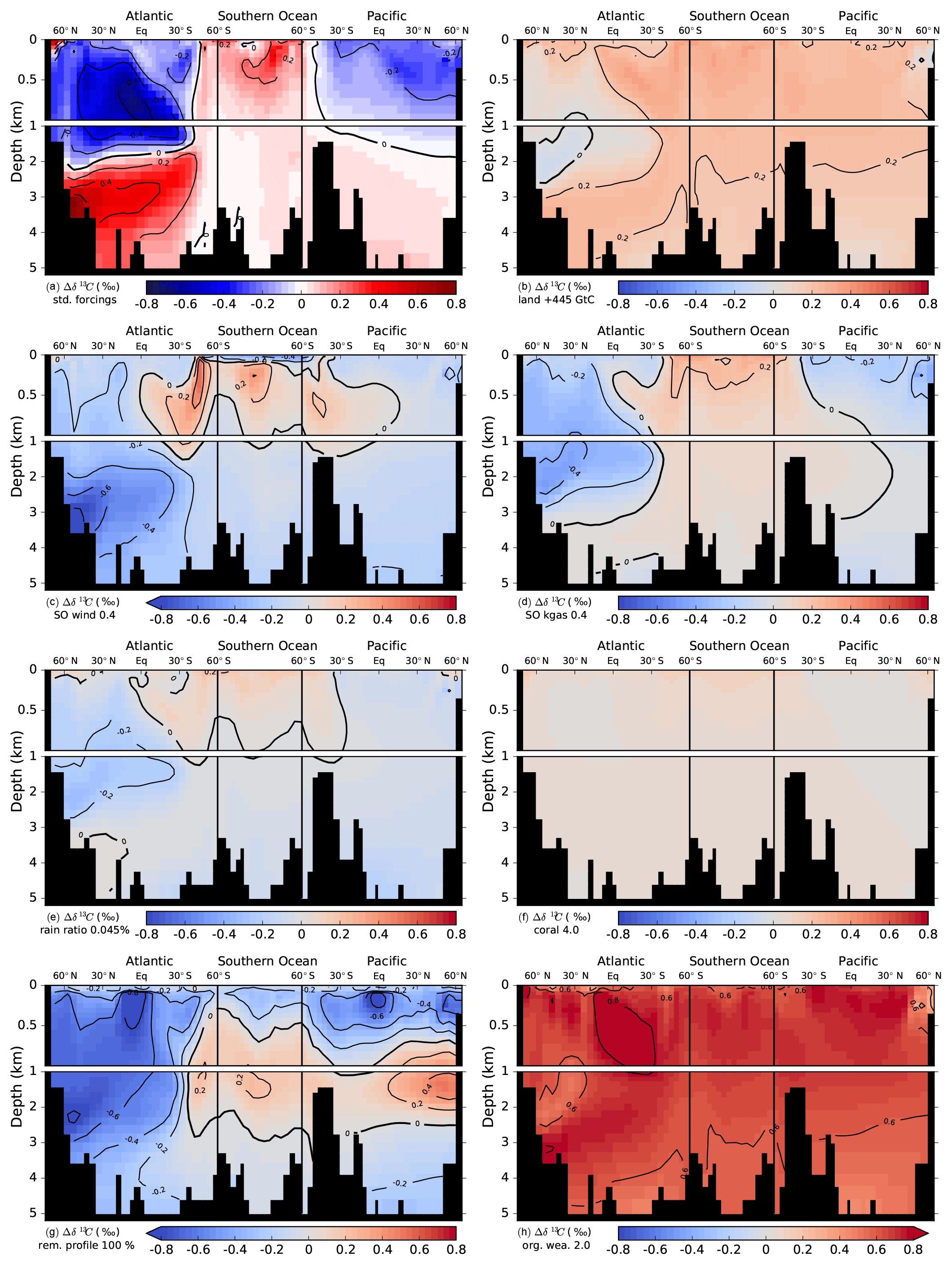
Figure 9Simulated deglacial change in the isotopic signature of DIC, Δδ13CDIC (PI minus LGM). Values are displayed along sections across the Atlantic, Southern Ocean, and Pacific and in response to standard deglacial forcings (b–h) due to changes in individual mechanisms as inferred from factorial simulations. Δδ13CDIC is shown for a deglacial carbon uptake of 445 GtC by the land biosphere (b), Southern Ocean wind stress (c), and gas transfer rate (d) scaled by a factor of 0.4 during the glacial relative to PI, rain ratio reduced to 0.045 during the glacial (e), deglacial shallow water carbonate deposition scaled by a factor of 4 (f), a change in the organic matter remineralization between a linear profile during the glacial and the standard depth scaling (g), and for a twofold increase in the organic weathering flux during the glacial compared to PI (h). The absolute change in Δδ13CDIC is shown in panel (a) for the standard forcings (bright colors), while panels (b) to (h) show the difference relative to the standard run (pastel colored).
The sensitivity simulations may be grouped by processes with small and large changes in the spatial pattern of Δδ13CDIC. Δland, coral reef regrowth, and organic weathering flux affect the input of carbon and carbon isotopes into the atmosphere–ocean system, leading to relatively uniform patterns of change (Fig. 9b, f, and h). Changes in SO wind stress, SO gas transfer rate, rain ratio, and upper ocean remineralization profile, on the other hand, mainly lead to a redistribution of carbon and carbon isotopes in the atmosphere–ocean system amplified by sediment interactions (Fig. 9c, d, e, g).
The uptake of carbon by the land biosphere leaves the atmosphere and ocean relatively enriched in δ13C (Fig. 9b). As a result of the carbon removal from the coupled system, changes in bottom water concentrations of and O2 may influence sedimentation fluxes of POC and CaCO3 locally and lead to small local patterns (see, for instance, negative anomalies in Δδ13CDIC in the North Atlantic deep water (NADW) region of Fig. 9b). Generally, though, a smooth pattern emerges for changes in Δland. Similarly, the doubling of the organic weathering flux during the glacial results in a strong uniform change in Δδ13CDIC (Figs. 9h and 7a). Increased rates of coral reef regrowth have little impact on Δδ13CDIC as the isotopic signature is similar for DIC and deposited CaCO3 (Fig. 9f). The slight increase in Δδ13CDIC in response to enhanced coral reef regrowth has been attributed to changes in fractionation during marine photosynthesis (Freeman and Hayes, 1992; Menviel and Joos, 2012).
Changes in the other four mechanisms affect the spatial pattern of Δδ13CDIC significantly (Fig. 9c, d, e, g). We note that these patterns result from adjustment processes acting on different timescales. We recall the forcing history for changes in Southern Ocean wind stress, Southern Ocean gas transfer rate, the rain ratio, the remineralization profile, and the organic weathering rate; PI values are set to LGM values at 40 ka, kept constant from 40 to 18 ka, scaled back to the PI value over the termination (18 to 11 ka), and kept constant thereafter (see also Fig. 3 and Table 2). Results are therefore not directly comparable to the step-change experiments described by Tschumi et al. (2011). As discussed in detail by Tschumi et al. (2011) and Menviel et al. (2015), a more poorly ventilated ocean due to reduced wind stress leads to an increase in δ13Catm. Changes in temperature and circulation in response to decreased Southern Ocean wind stress at the beginning of our simulation (Fig. 3f) lead to lower marine oxygen concentrations and an increase in POC sedimentation. Subsequent removal of 13C-depleted carbon from the ocean increases δ13CDIC. Restoring wind stress to its initial value over the deglacial reverses the changes. As the sediment feedbacks act on longer timescales, propagation of the signal to the whole ocean is not yet achieved. A complex interplay of processes, such as changes in circulation and subsequent changes in export fluxes, oxygen concentrations, and remineralization of POC, as well as changes in the lysocline and CaCO3 cycling spatially, overlay each other, yielding the Δδ13CDIC distribution seen in Fig. 9C.
Ocean–sediment interactions also play an important role for δ13CDIC in the case of changes in the Southern Ocean gas transfer rate. Decreasing the gas transfer rate at the beginning of the 40 kyr simulation (Fig. 3f) leads to a strong increase in δ13Catm. The ocean–sediment interactions are very similar to those described for SO wind stress changes above. The sedimentation fluxes of POC and CaCO3 increase in response to reduced oxygen concentrations from a lower gas transfer rate and changes in the concentration, as does the δ13C signature of the flux, leading to a removal of 13C from the ocean. From LGM to PI the opposite process takes places (increasing gas transfer back to its initial value); however, due to the long timescales of ocean–sediment interactions, the signal has not propagated to the whole ocean, and in the Atlantic and Pacific negative Δδ13CDIC still prevails (Fig. 9d).
As discussed in detail in Tschumi et al. (2011), responses in δ13C from reducing the export rain ratio are small in both the ocean and atmosphere (Fig. 7a–b) and arise from weathering–sedimentation imbalances and changes in the isotopic value of CaCO3 and POC. This negative perturbation in δ13C is not removed entirely over the deglacial and Holocene due to the long ocean–sediment response timescale, leaving the generally negative Δδ13CDIC as seen in Fig. 9e.
Finally, a change to a linear remineralization profile in the upper 2 km during the glacial leads to a dipole pattern in δ13CDIC with enriched values in the upper 1 km of the ocean and depleted values underneath (not shown). Across the deglacial, the process is reversed, yielding the pattern in Δδ13CDIC seen in Fig. 9g from the overlap of different response timescales. Applied changes in the remineralization profile lead to loss of carbon from the atmosphere–ocean system from LGM to PI.
In summary, the carbon and carbon isotope balance in our model simulations can change as a result of altered input fluxes, changes in the surface ocean δ13C signatures, which are then reflected in POC and CaCO3 export fluxes and coral reef regrowth, and altered sedimentation fluxes as a result of altered bottom water and O2 concentrations. For all seven mechanisms, weathering–sedimentation imbalances and feedbacks exert an impact on the carbon and carbon isotope budget and need to be taken into account on glacial–interglacial timescales. Also, the overlap of different response timescales for atmosphere–ocean and ocean–sediment interactions shapes the patterns in Δδ13CDIC.
We show that carbon exchange with ocean sediments and the lithosphere biases earlier δ13C-based estimates of deglacial change in land carbon storage towards lower values. This finding appears very robust considering modern estimates and reconstructions of ocean–sediment and weathering fluxes and our understanding of the marine carbonate chemistry. Many earlier estimates of land carbon storage change rely on the budget of the stable carbon isotope but neglected the isotopic exchange fluxes with marine sediments and the lithosphere. This approach became popular, perhaps as it is simple and transparent to solve two global budget equations. However, results from idealized pulse–release experiments as well as from transient deglacial simulations show that this neglect is not justified. Several processes that were potentially important for the reorganization of the deglacial carbon cycle influence the mean ocean δ13C signature significantly. Their influence cannot be ignored when analyzing the budget of δ13C on deglacial timescales. The importance of ocean sediment and lithosphere fluxes in regulating past atmospheric CO2 and carbon, isotopes, nutrient, and alkalinity inventories in the ocean is also emphasized in previous modeling studies (e.g., Huybers and Langmuir, 2009; Tschumi et al., 2011; Roth and Joos, 2012; Roth et al., 2014; Wallmann et al., 2015; Heinze et al., 2016). Data-based reconstructions of burial fluxes of calcium carbonate and organic matter (Cartapanis et al., 2016, 2018) reveal that these fluxes are more dynamic than previously assumed.
4.1 Uncertainties of this study
There are a number of uncertainties in our approach. We rely on characteristic forcing–response relationship as obtained with the Bern3D model, and these may be different than in reality. The current crop of models, including the Bern3D model, is not able to freely simulate reconstructed variations in atmospheric CO2 and other biogeochemical variables over the deglacial period. Nevertheless, the Bern3D model simulates the modern distribution of a range of water mass, ventilation, and biogeochemical tracers in good agreement with observational data (Roth et al., 2014). Global inventories and spatial distributions of biogenic CaCO3, organic carbon, and opal in the sediments, as well as their fluxes between the ocean, marine sediments, and the lithosphere are in agreement with preindustrial data-based estimates (see Appendix B and Table 1). The Bern3D model simulates a weaker and shallower Atlantic meridional overturning circulation at the LGM compared to the PI, and the simulated anomalies in δ13C of DIC agree with corresponding reconstructions (see Fig. 9 in Menviel et al., 2012). Regarding dissolved oxygen, qualitative reconstructions show a general decrease in oxygenation at intermediate depths and increase in the deep ocean (Jaccard and Galbraith, 2012; Jaccard et al., 2014; Galbraith and Jaccard, 2015) across the deglaciation. This pattern is also reproduced (not shown) in Bern3D model simulations.
We selected a set of seven generic, archetypical processes that are varied in deglacial simulations in addition to the processes explicitly implemented in the Bern3D model. These archetypical processes are intended to represent the space of multi-proxy response relationships (Fig. 8) for all the different processes that plausibly influenced deglacial carbon cycle changes. This is a simplification, though we argue that the seven selected processes roughly cover the plausible range of multi-proxy responses (Fig. 8). In addition, uncertainties in the importance of these processes are explicitly considered in our Monte Carlo approach and contribute to the uncertainty range in our estimate of Δland.
For example, there are various carbon reservoirs with an isotopic light signature very similar to that of plant and soil carbon. These include organic carbon stored in ocean sediments and shelves (Broecker, 1982; Ushie and Matsumoto, 2012; Cartapanis et al., 2016), dissolved organic carbon (DOC) in the ocean (Hansell, 2013), and gaseous CO2 stored in the unsaturated zones of aquifers from the decomposition of organic material (Baldini et al., 2018). Any carbon release or uptake from these reservoirs might be wrongly attributed to a change in the carbon inventory of the land biosphere given their very similar δ13C signature and similar multi-proxy response relationships. Indeed, changes in these reservoirs have been invoked as an alternative explanation for the reconstructed deglacial change in marine δ13C (Broecker, 1982; Zimov et al., 2006, 2009; Zech et al., 2011; Kemppinen et al., 2018). The deglacial change in CO2 stored in the unsaturated zone of aquifers is in the range of 12 to 86 GtC (Baldini et al., 2018) and is small compared to the estimated change in land carbon of around 850 GtC. Perhaps more important, the modern inventory of refractory DOC is about 650 GtC (Hansell, 2013) and assumed constant in Bern3D, while changes in the small inventory of labile DOC are explicitly simulated. It is unclear how the DOC pool varied over the past. Further, Cartapanis et al. (2016) suggest an approximately linear decrease in the flux of organic carbon transferred to deep ocean sediments from around 28 GtC kyr−1 at the LGM to around 17 GtC kyr−1 during the Holocene, corresponding to a cumulative imbalance of around 55 GtC. The change in organic carbon stocks stored in sediments on shelves is uncertain and may amount to several hundred gigatons of carbon over the deglaciation. Here, we varied organic-like carbon input by weathering in the unconstrained ensemble over a range corresponding to a cumulative PI–LGM anomaly of +780 to −1560 GtC. These anomalies in input, though not directly comparable to inventory changes, are large in comparison to the inventory changes discussed here. In summary, a potential misattribution of changes in other organic carbon reservoirs to changes in Δland is included in our uncertainty estimate of Δland.
Our approach is limited in that we only consider the change between LGM and PI for four relevant proxy variables. This restriction allowed us to build a cost-efficient and nonlinear emulator to explore a very large range of parameter combinations. Future efforts to refine estimates of Δland may explicitly consider the spatial and temporal evolution for a large number of proxies.
4.2 Contribution of deglacial mechanisms to the CO2 rise
Turning to the role of different mechanisms for the deglacial increase in atmospheric CO2, we find that ocean circulation changes only partly explain the deglacial CO2 rise. Ocean circulation changes are not able to simultaneously explain glacial–interglacial changes in δ13CDIC and CO2 in our model (see Fig. 8a), in agreement with earlier studies (e.g., (Tschumi et al., 2011; Heinze et al., 2016)).
A modest and plausible (Bendtsen et al., 2002; Matsumoto, 2007) deepening of the remineralization of organic matter in the upper ocean (see Fig. C2e) leads to large changes in atmospheric CO2, while at the same time hardly changing deep Pacific . This also holds for other biological mechanisms such as an increased nutrient utilization in response to iron fertilization or an elevated phosphorus input to the ocean (Menviel et al., 2012). This renders this class of processes potentially important to explain part of the deglacial CO2 increase, as reconstructions suggest small LGM to PI changes in deep Pacific concentrations (Yu et al., 2014). Accordingly, in all Monte Carlo realizations the remineralization depth of organic matter is deeper at the LGM than PI in our approach.
Our solutions also point to a significant role of alkalinity-based mechanisms for the deglacial CO2 increase (see Fig. C2d). The constrained ensemble yields a large extra burial of CaCO3 as well as an increase in the rain ratio of CaCO3 to organic matter by particle export over the deglaciation. This is qualitatively consistent with the reconstruction of Cartapanis et al. (2018), who suggest that the CaCO3 burial flux (below 200 m) increased by about 0.2 GtC yr−1 from the LGM to the Holocene.
4.3 Comparison to other estimates of Δland
Δland estimates range from −400 GtC, e.g., a larger terrestrial carbon inventory during the glacial (Zimov et al., 2006, 2009; Zech et al., 2011; Kemppinen et al., 2018), to 1500 GtC (Adams and Faure, 1998) based on a variety of methods. The low end is based on reconstructions of the carbon content in paleosols (Zimov et al., 2006, 2009; Zech et al., 2011). These reconstructions are scarce, of local nature, and restricted to cold high-altitude or high-latitude regions, rendering extrapolations to the global scale speculative. In a recent data synthesis, Lindgren et al. (2018) suggest that the loss of carbon from Northern Hemisphere permafrost from the LGM to PI was lower than initially suggested by Zimov et al. (2009) and that total land carbon storage in northern middle and high latitudes increased by about 400 GtC over the deglaciation. Kemppinen et al. (2018) suggest a negative Δland based on results from an Earth system model of intermediate complexity. However, these authors did not consider any isotopic constraints. Our results suggest negative Δland values to be highly unlikely and Δland to be likely larger than 450 GtC. Otherwise, solutions for δ13CDIC are significantly biased low compared to the data-based reconstruction.
The high end of the Δland range, implying much smaller land carbon storage during the LGM than today, is based on estimates relying on pollen records (Adams et al., 1990; Van Campo et al., 1993; Crowley, 1995; Adams and Faure, 1998). Pollen and macrofossils recorded in various archives hold information on past vegetation distribution but do not allow for constraining carbon inventories in soils or in vegetation, rendering the derivation of Δland estimates based on pollen data difficult (Hoogakker et al., 2016). Ice core CO2 and δ13Catm records constrain the preindustrial terrestrial carbon uptake over the Holocene to about 250 GtC (Elsig et al., 2009). Assuming the total estimate of 1500 GtC by Adams and Faure (1998) was right, this would leave more than 1200 GtC to be transferred to the terrestrial biosphere between the LGM and the beginning of the Holocene. Considering possible processes that could achieve such a large transfer seems difficult. Generally this might pose an upper limit to Δland.
Our estimate of Δland appears consistent with a recent biome-based reconstruction of soil carbon storage (Lindgren et al., 2018). Lindgren et al. (2018) report an increase in soil carbon inventory of about 400 GtC for the region north of about 30∘ N and considering changes in permafrost, mineral, and peatland, as well as in loess and subglacial soil. This is in agreement with our Δland estimate when assuming an increase in carbon stored in vegetation and in tropical and Southern Hemisphere ecosystems and soils. Furthermore, modeling studies have generally yielded positive Δland estimates of about 400–900 GtC (Joos et al., 2004; Prentice et al., 2011; Brovkin et al., 2012; O'Ishi and Abe-Ouchi, 2013; Ganopolski and Brovkin, 2017; Davies-Barnard et al., 2017).
In summary, many lines of evidence point to a positive Δland, and we suggest a likely range of about 450 to 1250 GtC. Yet, the uncertainty in this estimate remains large owing to both uncertainties in processes and in observational constraints. Unfortunately, the necessity of including exchange with sediments and the lithosphere and other deglacial processes in the isotopic budget adds complexity. This tends to increase the uncertainty range compared to simplified and biased assessments that consider the isotopic budget in the closed ocean–land–atmosphere system.
We used a Bayesian approach to constrain the change in the land biosphere carbon inventory between the Last Glacial Maximum and the preindustrial period. Four data-based constraints are applied: the deglacial change in the δ13C signature of atmospheric CO2 and of dissolved inorganic carbon in the ocean; and the deglacial change in atmospheric CO2 and in deep Pacific carbonate ion concentrations. The strength of generic, archetypical mechanisms for deglacial biogeochemical changes was varied in 500 000 simulations in an emulator built from a large suite of Bern3D model simulations. Carbon, nutrient, alkalinity, and carbon isotope exchange with the lithosphere and ocean sediments is explicitly taken into account, in contrast to earlier studies that applied the isotopic budget of 13C to estimate deglacial change in land biosphere carbon.
We demonstrate in idealized and transient deglacial simulations that isotopic exchange with ocean sediments and the lithosphere is important for the budget of 13C on timescales of the deglaciation. We find that the carbon stocks in the land biosphere were likely around 450 to 1250 GtC (±1 standard deviation) larger at preindustrial times than at the Last Glacial Maximum. The median estimate is ∼850 GtC. This is much larger than earlier estimates based on the budget of the stable carbon isotope 13C. These earlier studies neglected interactions with the lithosphere and ocean sediments and the influence of other deglacial carbon cycle processes on the isotopic budget. This neglect biases their estimate significantly low. Our multi-proxy approach suggests that a combination of different mechanisms contributed to the deglacial increase in CO2. These include, aside from ocean circulation, temperature and salinity changes, a net removal of alkalinity from the surface ocean through increased burial of calcium carbonate in coral reefs and ocean sediments, and potentially increasing export of calcium carbonate from the surface to the deep ocean. Further, changes in biological mechanisms such as a deglacial shoaling of the remineralization depth for organic matter may have been instrumental in increasing atmospheric CO2. The results demonstrate that ocean sediments and the weathering–burial cycle are an integral part of the Earth system playing a fundamental role on glacial–interglacial timescales.
Data used for this study are available upon request to the corresponding author (jeltsch@climate.unibe.ch).
A1 The Bern3D model
The Bern3D EMIC features a three-dimensional geostrophic ocean (Müller et al., 2006; Edwards et al., 1998) with an isopycnal diffusion scheme and Gent–McWilliams parameterization for eddy-induced transport (Griffies, 1998). The model includes a thermodynamic sea-ice component coupled to a single-layer energy–moisture balance atmosphere (Ritz et al., 2011). Further, a sediment module (Tschumi et al., 2011; Heinze et al., 1999) and a four-box terrestrial biosphere (Siegenthaler and Oeschger, 1987) are coupled to the model.
The horizontal resolution is 41×40 grid cells (Roth et al., 2014; Battaglia and Joos, 2018a, b) and is the same for the ocean, atmosphere, and sea-ice components. In the vertical, the ocean has 32 logarithmically spaced layers. Wind stress at the surface is prescribed following the NCEP/NCAR monthly wind stress climatology (Kalnay et al., 1996). Carbonate chemistry and the air–sea gas exchange for CO2 and 14CO2 are implemented according to OCMIP-2 protocols (Najjar and Orr, 1999; Orr et al., 1999) with updates for the 14C standard ratio and half-life (Orr et al., 2017), the calculation of the Schmidt number (Wanninkhof, 2014), and the carbonate chemistry (Orr and Epitalon, 2015). In order to match observational estimates of natural and bomb-produced 14C, the global mean air–sea transfer is reduced by 19 % compared to OCMIP-2 in order to match observation-based radiocarbon estimates (Müller et al., 2008). Another update with respect to the OCMIP-2 protocols concerns the gas transfer velocity, which scales linearly with wind speed following Krakauer et al. (2006). Analog and consistent formulations are used for air–sea exchange of oxygen and 13CO2.
Biogeochemical cycling in the model is detailed in Tschumi et al. (2011) and Parekh et al. (2008) with further documentation of results in follow-up studies (e.g., Menviel et al., 2012, 2015; Menviel and Joos, 2012; Roth and Joos, 2012; Roth et al., 2014; Battaglia et al., 2016; Battaglia and Joos, 2018b, a). Dissolved inorganic carbon and semi-labile organic carbon (DIC, DOC), the corresponding isotopic forms (DI13C, DO13C, DI14C, DO14C), and alkalinity (Alk), phosphate (PO4), oxygen (O2), iron (Fe), silica (Si), and an ideal age tracer are explicitly transported by advection, diffusion, and convection. New production of organic matter is limited to the euphotic zone in the uppermost 75 m and calculated as a function of light availability, temperature, and phosphate and iron availability (Doney et al., 2006). Bacteria and plankton are not explicitly represented. Two-thirds of the new production is transferred to the pool of dissolved organic carbon (DOC) and the remainder is exported as particulate organic carbon (POC) (Tschumi et al., 2008). The biological fluxes of C, PO4, Alk, and O2 and the corresponding elemental ratios in DOC and POC are linked by fixed Redfield ratios (; Sarmiento and Gruber, 2006). DOC decays with a lifetime of 0.5 yr. POC is remineralized following a Martin's curve (Martin et al., 1987) given by
where z0 refers to the reference depth of 75 m (see also Roth et al., 2014). Export of calcium carbonate (CaCO3) and of opal is computed from new production and availability of dissolved silica in the euphotic zone. The export rain ratio of CaCO3 to POC is set to 0.083 in the absence of dissolved silica, while the production ratio of CaCO3 to POC is reduced at the favor of opal production in regions with abundant availability of silicic acid. Particulate CaCO3 and opal are remineralized below the euphotic zone with an e-folding depth scale of 5066 and 10 000 m, respectively.
A 10-layer sediment diagenesis module (Tschumi et al., 2011; Heinze et al., 1999) is used to explicitly calculate transfer fluxes to and redissolution fluxes from reactive sediment to the water column as well as loss fluxes to the lithosphere for nutrients, carbon, and carbon isotopes. In equilibrium, loss fluxes to the lithosphere are equal to input fluxes by weathering. The sediment module dynamically calculates the transport, redissolution, remineralization, and bioturbation of solid material, the pore-water chemistry, and diffusion in the top 10 cm of the sediment. Four solid tracers (CaCO3, opal, POC, clay) and seven tracers in the pore water (DIC, DI13C, DI14C, alkalinity, phosphate, oxygen, and silicic acid) are modeled. The dissolution of CaCO3 depends on the pore-water concentration. The oxidation rate of POC, on the other hand, depends on oxygen concentrations in the pore water and the weight fraction of POC in the solid phase of the sediment. Denitrification is not considered in this model version, but O2 is not consumed below a threshold, somewhat reflecting the process of denitrification without modeling . The respective reaction rate parameters for CaCO3 dissolution and POC oxidation are global constants (see Roth et al., 2014). The model assumes conservation of volume; i.e., the entire column of the sediments is pushed downwards if deposition exceeds redissolution into pore waters. Any solid material that is pushed out of the diagenetic zone (top 10 cm) disappears into the subjacent diagenetically consolidated zone (burial or loss flux) (see Tschumi et al., 2011, for more details). Carbonate chemistry within sediment pore waters is calculated as in the ocean by using the MOCSY routine of Orr and Epitalon (2015).
Weathering fluxes of PO4, Alk, DIC, DI13C, and silicic acid are added uniformly to the coastal surface ocean. The global weathering fluxes are set equal to the burial fluxes diagnosed at the end of the model spin-up. In the standard model setup these diagnosed input fluxes are kept constant. The pulse experiments include a setting in which the input fluxes vary as a function of global mean surface air temperature and CO2 following Colbourn et al. (2013). One of the factorial sensitivity runs assesses the impact of altered input fluxes of organic material across the deglacial. This weathering–burial cycle and the associated burial–nutrient feedbacks (Tschumi et al., 2011) are important for the mass balance of 13C and for the removal of marine perturbations in nutrients, carbon, and isotopes on deglacial timescales. In other words, these processes directly affect the estimate of the change in land carbon from the 13C mass balance.
The atmosphere exchanges carbon and carbon isotopes with a four-box land biosphere model (Siegenthaler and Oeschger, 1987). It includes a mass of 2220 GtC and represents the carbon that is actively exchanged with the atmosphere. This four-box reservoir is only used to simulate the dilution of an atmospheric isotopic perturbation by the land biosphere but not to address changes in land carbon stocks. The carbon inventory of the land biosphere, and thus the dilution of an isotopic perturbation, is about 20 times smaller than that of the ocean–atmosphere–sediment system.
13C stocks and flows are modeled in the atmosphere–ocean–sediment–land biosphere system. 13C fluxes to the lithosphere associated with the burial of POC and CaCO3 and weathering input are explicitly simulated. 13C fractionation is considered for air–sea gas transfer, carbonate chemistry, the formation of CaCO3, POC, DOC, and photosynthesis on land, while no fractionation is assumed during remineralization on land and in the ocean. Gross air-to-sea and gross sea-to-air fluxes of 13CO2 are implemented considering kinetic fractionation (Siegenthaler and Oeschger, 1987) and strongly temperature–dependent equilibrium fractionation between the various carbonate species (Mook, 1986). Isotopic fractionation during CaCO3 formation is small and computed following Mook (1986). This results in an isotopically heavy signature of around 2.9 ‰ for CaCO3. Fractionation during photosynthesis in the ocean and thus between dissolved CO2 ([CO2]) and POC and DOC is calculated according to Freeman and Hayes (1992). The fractionation increases logarithmically with [CO2] in surface water and results in an isotopically light signature for POC and DOC of around −20 ‰. A lowering of [CO2], or correspondingly of pCO2, by about 10 % yields a change in the isotopic signature of POC by +0.55 ‰. The burial of POC and CaCO3 results in an isotopic signature of the burial flux of around −9 ‰, intermediate between the isotopically light POC and the isotopically heavy CaCO3 signature. In equilibrium, the burial flux is compensated for by a weathering input flux of equal amount and signature. On land, a constant fractionation of 18.1 ‰ is applied for simplicity.
A2 Initialization of Bern3D simulations
The model is spun up over 60 000 years to a preindustrial equilibrium corresponding to 1765 CE boundary conditions similar to the approach outlined in Roth et al. (2014). CO2 is set to 278 ppm and δ13C of CO2 to −6.305 ‰. The loss of tracers due to sedimentary burial is compensated for during the spin-up by variable weathering fluxes in order to conserve oceanic inventories of tracers. After the system has equilibrated, the weathering fluxes are kept constant at the values diagnosed at the end of the spin-up in the standard setup.
A3 Bern3D pulse experiments
Idealized experiments with a pulse-like carbon removal from the atmosphere are conducted in (i) a closed system, (ii) an open system, and (iii) an open system model configuration allowing for weathering feedbacks. In (i), only the atmosphere–ocean–land biosphere model components are used and all tracers are conserved within these three reservoirs. In (ii), the sediment module is added to the configuration outlined above and the carbon and tracer inventories within the atmosphere–ocean–land biosphere system are allowed to vary due to weathering–burial imbalances. In (iii), weathering fluxes vary in response to changes in atmospheric temperature and CO2 concentrations following the parameterizations given in Colbourn et al. (2013), accounting for changes in CaCO3 and CaSiO3 weathering on land.
Simulations are started from the end of the PI spin-up, and atmospheric CO2 and δ13C are computed in a prognostic way based on air–sea and air–land fluxes. In year 100 of the simulation, 100 GtC of carbon with a δ13C signature of −24 ‰ is instantaneously removed from the atmosphere, mimicking an immediate regrowth of the terrestrial biosphere. After the pulse, the model is run for 100 kyr and anomalies are expressed relative to a control run. Control simulations show negligible changes in CO2 and δ13C as model drift is small.
The implied change in the land biosphere carbon stock based on a closed system assumption is calculated for all three model settings by solving the following equations for ΔMTER, i.e., Δland:
with M representing the inventory, δ the isotopic signature, Δ the respective time interval, and the subscripts A, B, and O referring to the atmosphere, terrestrial biosphere, and ocean, respectively. The calculated Δland is then compared to the prescribed carbon uptake. This allows us to investigate the validity of the closed system assumption on different timescales.
The aim of the sediment tuning was to improve the representation of export, deposition, and dissolution fluxes of POC, CaCO3, and opal, as well as the distribution of weight fractions of these tracers in the sediment module of the Bern3D model after the change of the horizontal model resolution introduced in Roth et al. (2014). One concern was the total amount of CaCO3 in the reactive uppermost 10 cm of the sediment represented in the sediment module. Prior to tuning, the global CaCO3 content in the model was ∼400 GtC. Using observational constraints on modern global bulk mass accumulation rates (MARs) (Cartapanis et al., 2016), global carbonate MAR (Dunne et al., 2012; Jahnke, 1996), and the density, bulk sediment, and porosity in the uppermost 10 cm as used in the model, we estimate a target CaCO3 stock of ∼1000 GtC. The second concern was the opal burial that used to be ∼3 Tmol Si yr−1 but with new observational data suggesting a burial flux of ∼6.5 Tmol Si yr−1 (Tréguer and De La Rocha, 2013). Further, all other sediment-related fluxes of POC, CaCO3, and opal were tuned with regard to observational constraints (see Table 1).
Table B1Old and new parameter values in the Bern3D model that were varied in the tuning of the sediment component.
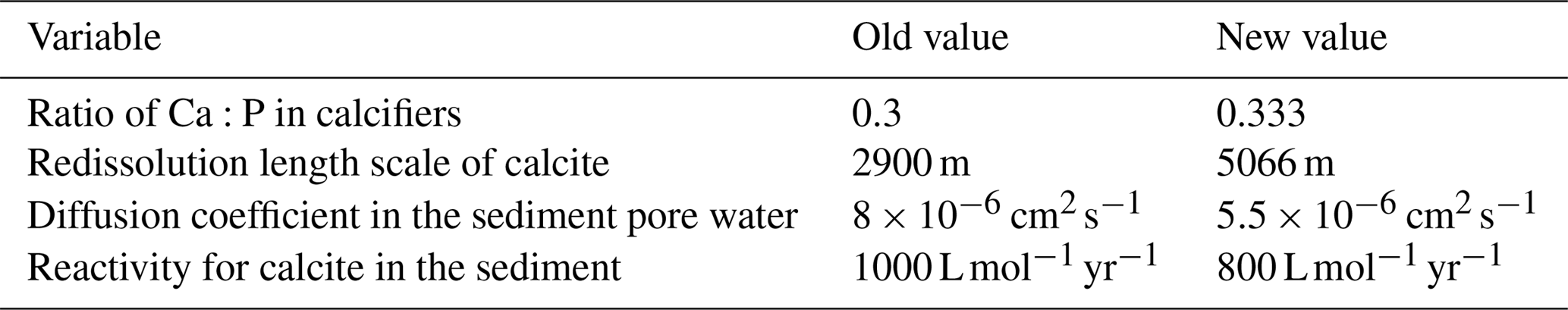
The tuning was carried out in two steps. In the first step, three parameters were varied: the ratio of Ca:P in calcifiers, the redissolution length scale for the calcite profile, and the reactivity for calcite in the sediment. In the second step, the reactivity of calcite and the diffusion coefficient in the sediment pore water were varied. For both steps, a 100-member LHS ensemble was run and skill scores calculated as outlined in Steinacher et al. (2013). For the calculation of the skill scores, ocean data from GLODAP v.2 (Lauvset et al., 2016) and the World Ocean Atlas 2013 version 2 (Locarnini et al., 2013; Zweng et al., 2013; Garcia et al., 2013a, b) datasets were used. For export, deposition, and burial of POC, CaCO3, and opal values from Battaglia et al. (2016), Tréguer and De La Rocha (2013), Sarmiento and Gruber (2006), Milliman and Droxler (1996), and Feely et al. (2004) were used. For the sediment data compilations by Cartapanis et al. (2016, 2018) were used to compare the model performance. The distribution of CaCO3 in the sediments after the tuning compared to observational data is shown in Fig. B1. Export, deposition, and burial fluxes for POC, CaCO3, and opal and the global sediment inventories in the model with respective observational ranges from the literature are given in Table 1 and the old and new parameter values in Table B1. The distribution of other tracers is comparable to before and as outlined in Roth et al. (2014).
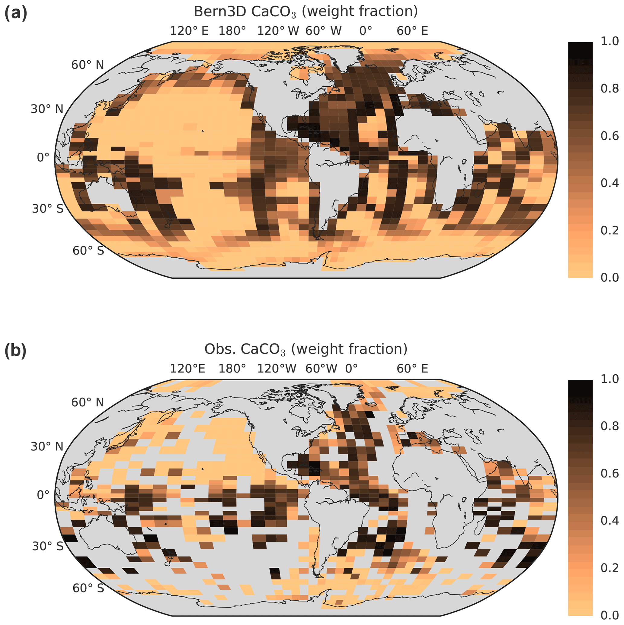
Figure B1(a) Distribution of CaCO3 in the Bern3D model after tuning of the sediment component under preindustrial boundary conditions compared to (b) sediment core-top CaCO3 data (Cartapanis et al., 2018). Core-top data were gridded onto the Bern3D grid and are a mean of the top 10 cm over the past 6 kyr. Grey indicates land (within coastlines) or missing data.
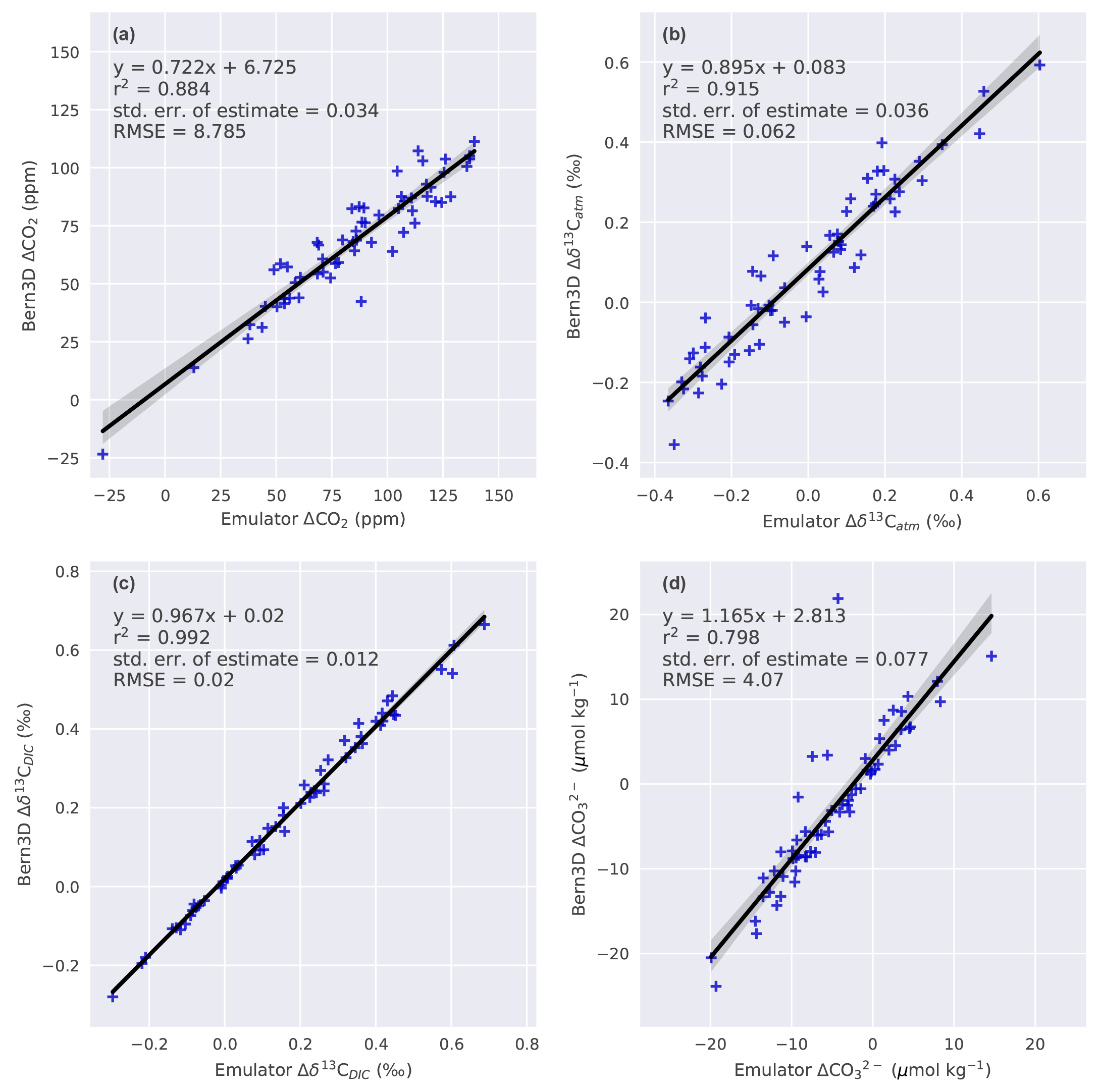
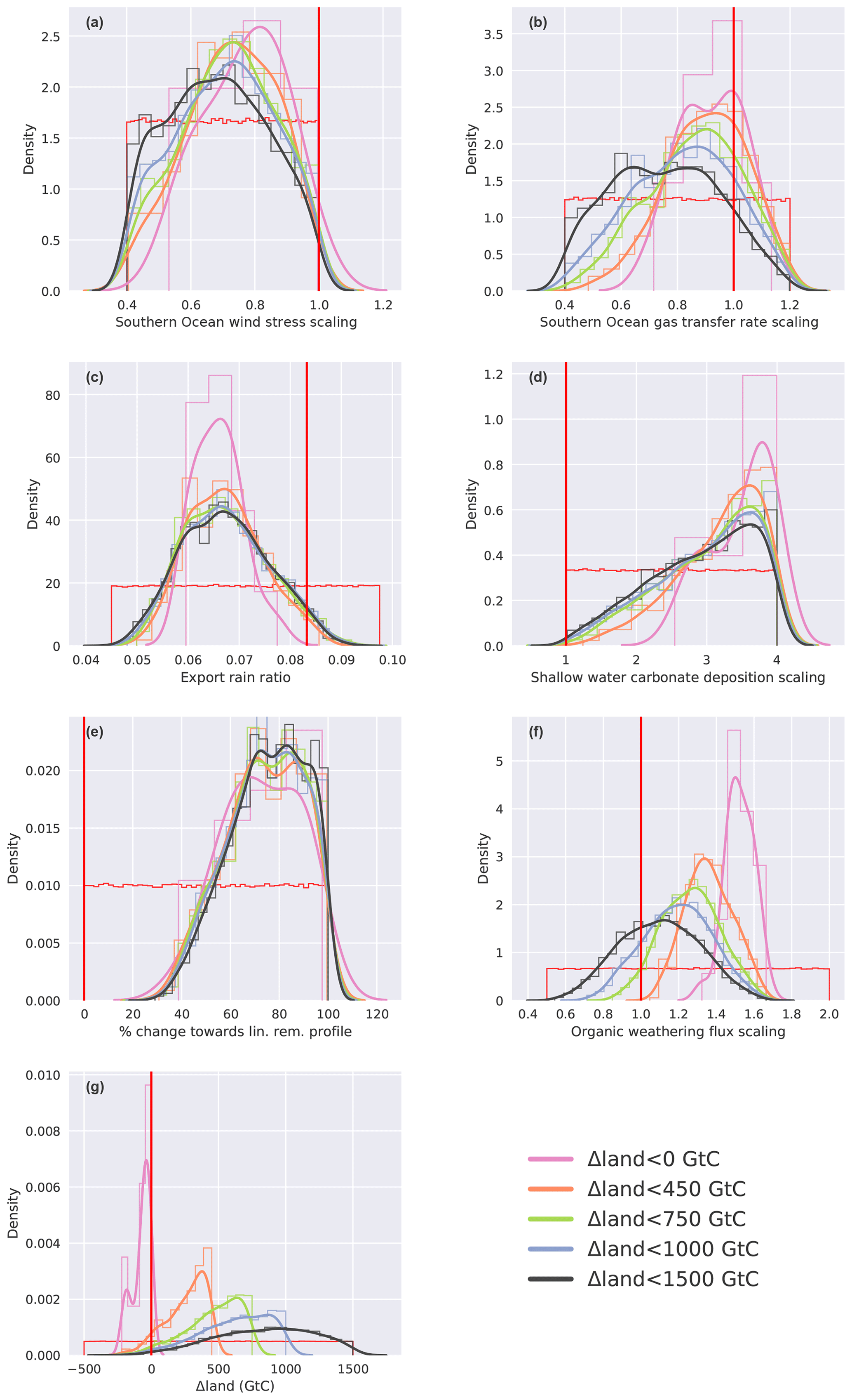
Figure C2Histograms (colored thin line, normalized) and kernel density estimates (colored thick line) of applied changes in the seven mechanisms (a–g) for all emulator results that fulfill the four observational constraints. The colors of the lines correspond to subsamples of these results according maximum changes in Δland of 1500, 1000, 750, 450, and 0 GtC. The thin red line gives the histogram of the prior distribution and the vertical thick red line the standard parameter value. For details on the mechanisms see Sect. 2.2.
The authors declare that they have no conflict of interest.
This article is part of the special issue “The 10th International Carbon Dioxide Conference (ICDC10) and the 19th WMO/IAEA Meeting on Carbon Dioxide, other Greenhouse Gases and Related Measurement Techniques (GGMT-2017) (AMT/ACP/BG/CP/ESD inter-journal SI)”. It is a result of the 10th International Carbon Dioxide Conference, Interlaken, Switzerland, 21–25 August 2017.
Aurich Jeltsch-Thömmes and Fortunat Joos acknowledge support by the Oeschger Centre for Climate Change Research and Gianna Battaglia and Fortunat Joos by the Swiss National Science Foundation (200020-172476). Olivier Cartapanis and Samuel L. Jaccard were funded by the Swiss National Science Foundation (grants PP00P2-144811 and PP00P2-172915).
This paper was edited by Helen McGregor and reviewed by Katsumi Matsumoto and one anonymous referee.
Adams, J. M. and Faure, H.: A new estimate of changing carbon storage on land since the last glacial maximum, based on global land ecosystem reconstruction, Glob. Planet. Change, 16/17, 3–24, 1998. a, b, c, d
Adams, J. M., Faure, H., Faure-Denard, L., McGlade, J. M., and Woodward, F. I.: Increases in terrestrial carbon storage from the Last Glacial Maximum to the present, Nature, 348, 711–714, 1990. a, b
Adkins, J. F.: The role of deep ocean circulation in setting glacial climates CO2, Paleoceanography, 28, 539–561, https://doi.org/10.1002/palo.20046, 2013. a
Archer, D. and Maier-Reimer, E.: Effect of deep-sea sedimentary calcite preservation on atmospheric CO2 concentration, Nature, 367, 260–263, https://doi.org/10.1038/367260a0, 1994. a
Archer, D., Khesgi, H., and Maier-Reimer, E.: Dynamics of fossil fuel CO2 neutralization by marine CaCO3, Global Biogeochem. Cy., 12, 259–276, 1998. a
Archer, D., Winguth, A., Lea, D., and Mahowald, N.: What caused the glacial/interglacial atmospheric pCO2 cycles?, Rev. Geophys., 38, 159–189, 2000. a, b, c, d
Armstrong, R. A., Lee, C., Hedges, J. I., Honjo, S., and Wakeham, S. G.: A new, mechanistic modelfor organic carbon fluxes in the ocean based on the quantitative association of POC with ballast minerals, Deep-Sea Res. Pt. II, 49, 219–236, 2002. a
Baldini, J. U., Bertram, R. A., and Ridley, H. E.: Ground air: A first approximation of the Earth's second largest reservoir of carbon dioxide gas, Sci. Total Environ., 616/617, 1007–1013, https://doi.org/10.1016/j.scitotenv.2017.10.218, 2018. a, b
Battaglia, G. and Joos, F.: Marine N2O Emissions From Nitrification and Denitrification Constrained by Modern Observations and Projected in Multimillennial Global Warming Simulations, Global Biogeochem. Cy., 32, 92–121, https://doi.org/10.1002/2017GB005671, 2018a. a, b
Battaglia, G. and Joos, F.: Hazards of decreasing marine oxygen: the near-term and millennial-scale benefits of meeting the Paris climate targets, Earth Syst. Dynam., 9, 797–816, https://doi.org/10.5194/esd-9-797-2018, 2018b. a, b
Battaglia, G., Steinacher, M., and Joos, F.: A probabilistic assessment of calcium carbonate export and dissolution in the modern ocean, Biogeosciences, 13, 2823–2848, https://doi.org/10.5194/bg-13-2823-2016, 2016. a, b, c
Bendtsen, J., Lundsgaard, C., Middelboe, M., and Archer, D.: Influence of bacterial uptake on deep-ocean dissolved organic carbon, Global Biogeochem. Cy., 16, 74-1–74-12, https://doi.org/10.1029/2002GB001947, 2002. a, b
Bereiter, B., Eggleston, S., Schmitt, J., Nehrbass-Ahles, C., Stocker, T. F., Fischer, H., Kipfstuhl, S., and Chappellaz, J.: Revision of the EPICA Dome C CO2 record from 800 to 600 kyr before present, Geophys. Res. Lett., 42, 542–549, https://doi.org/10.1002/2014GL061957, 2015. a
Berger, A.: Long-Term Variations of Daily Insolation and Quaternary Climatic Changes, J. Atmos. Sci., 35, 2362–2367, https://doi.org/10.1175/1520-0469(1978)035<2362:LTVODI>2.0.CO;2, 1978. a
Berger, W. H.: Increase of carbon dioxide in the atmosphere during deglaciation: the coral reef hypothesis, Naturwissenschaften, 69, 87–88, https://doi.org/10.1007/BF00441228, 1982. a, b
Berger, W. H. and Keir, R. S.: Glacial-Holocene Changes in Atmospheric CO2 and the Deep-Sea Record, in: Climate Processes and Climate Sensitivity, edited by: Hansen, J. E. and Takahashi, T., Vol. 29, American Geophysical Union (AGU), Washington DC, 337–351, https://doi.org/10.1029/GM029p0337., 2013. a
Bird, M. I., Lloyd, J., and Farquhar, G. D.: Terrestrial carbon storage at the LGM, Nature, 371, 566–566, https://doi.org/10.1038/371566a0, 1994. a, b, c
Bird, M. I., Lloyd, J., and Farquhar, G. D.: Terrestrial carbon-storage from the last glacial maximum to the present, Chemosphere, 33, 1675–1685, https://doi.org/10.1016/0045-6535(96)00187-7, 1996. a, b
Broecker, W. S.: Glacial to Interglacial Changes in Ocean Chemistry, Prog. Oceanogr., 11, 151–197, 1982. a, b
Broecker, W. S. and Clark, E.: Glacial-to-Holocene Redistribution of Carbonate Ion in the Deep Sea, Science, 294, 2152–2155, 2001. a
Brovkin, V., Ganopolski, A., Archer, D., and Rahmstorf, S.: Lowering of glacial atmospheric CO2 in response to changes on oceanic circulation and marine biogeochemistry, Paleoceanography, 22, 1–14, https://doi.org/10.1029/2006PA001380, 2007. a
Brovkin, V., Ganopolski, A., Archer, D., and Munhoven, G.: Glacial CO2 cycle as a succession of key physical and biogeochemical processes, Clim. Past, 8, 251–264, https://doi.org/10.5194/cp-8-251-2012, 2012. a, b
Burke, A. and Robinson, L. F.: The Southern Ocean's Role in Carbon Exchange During the Last Deglaciation, Science, 335, 557–562, 2012. a
Cartapanis, O., Bianchi, D., Jaccard, S., and Galbraith, E. D.: Global pulses of organic carbon burial in deep-sea sediments during glacial maxima, Nat. Commun., 7, 10796, https://doi.org/10.1038/ncomms10796, 2016. a, b, c, d, e, f, g, h, i
Cartapanis, O., Galbraith, E. D., Bianchi, D., and Jaccard, S. L.: Carbon burial in deep-sea sediment and implications for oceanic inventories of carbon and alkalinity over the last glacial cycle, Clim. Past, 14, 1819–1850, https://doi.org/10.5194/cp-14-1819-2018, 2018. a, b, c, d, e, f
Ciais, P., Tagliabue, A., Cuntz, M., Bopp, L., Scholze, M., Hoffmann, G., Lourantou, A., Harrison, S. P., Prentice, I. C., Kelley, D. I., Koven, C., and Piao, S. L.: Large inert carbon pool in the terrestrial biosphere during the Last Glacial Maximum, Nat. Geosci., 5, 74–79, https://doi.org/10.1038/ngeo1324, 2012. a, b, c
Ciais, P., Sabine, C., Bala, G., Bopp, L., Brovkin, V., Canadell, J., Chhabra, A., DeFries, R., Galloway, J., Heimann, M., Jones, C., Le Quéré, C., Myneni, R. B., Piao, S., and Thornton, P.: Carbon and Other Biogeochemical Cycles, in: Climate Change 2013: The Physical Science Basis. Contribution of Working Group I to the Fifth Assessment Report of the Intergovernmental Panel on Climate Change, edited by: Stocker, T. F., Qin, D., Plattner, G.-K., Tignor, M., Allen, S. K., Boschung, J., Nauels, A., Xia, Y., Bex, V., and Midgley, P. M., Cambridge University Press, Cambridge, United Kingdom and New York, USA, 2013. a, b
Colbourn, G., Ridgwell, A., and Lenton, T. M.: The Rock Geochemical Model (RokGeM) v0.9, Geosci. Model Dev., 6, 1543–1573, https://doi.org/10.5194/gmd-6-1543-2013, 2013. a, b, c
Crowley, T. J.: Ice age carbon, Nature, 352, 575–576, 1991. a
Crowley, T. J.: Ice age terrestrial carbon changes revisited, Global Biogeochem. Cy., 9, 377–389, 1995. a, b
Curry, W. B., Duplessy, J. C., Labeyriefi, L. . D., and Shackleton, N. J.: Changes in the distribution of δ13C of deep water CO2 between the last glaciation and the Holocene, Paleoceanography, 3, 317–341, https://doi.org/10.1029/PA003i003p00317, 1988. a, b
Davies-Barnard, T., Ridgwell, A., Singarayer, J., and Valdes, P.: Quantifying the influence of the terrestrial biosphere on glacial-interglacial climate dynamics, Clim. Past, 13, 1381–1401, https://doi.org/10.5194/cp-13-1381-2017, 2017. a
Doney, S. C., Lindsay, K., Fung, I., and John, J.: Natural variability in a stable, 1000-yr global coupled climate-carbon cycle simulation, J. Clim., 19, 3033–3054, https://doi.org/10.1175/JCLI3783.1, 2006. a
Dunne, J. P., Hales, B., and Toggweiler, J. R.: Global calcite cycling constrained by sediment preservation controls, Global Biogeochem. Cy., 26, 1–14, https://doi.org/10.1029/2010GB003935, 2012. a
Duplessy, J. C., Shackleton, N. J., Matthews, R. K., Prell, W., Ruddimann, W. F., Caralp, M., and Hendy, C. H.: 13C Record of benthic foraminifera in the last interglacial ocean: Implications for the carbon cycle and the global deep water circulation, Quaternary Res., 21, 225–243, https://doi.org/10.1016/0033-5894(84)90099-1, 1984. a, b
Duplessy, J. C., Shackleton, N. J., Fairbanks, R. G., Labeyriefi, L., Oppo, D., Labeyrie, L., Oppo, D., and Kallel, N.: Deepwater source variations during the last climatic cycle and their impact on the global deepwater circulation, Paleoceanography, 3, 343–360, https://doi.org/10.1029/PA003i003p00343, 1988. a
Edwards, N. R., Willmott, A. J., and Killworth, P. D.: On the Role of Topography and Wind Stress on the Stability of the Thermohaline Circulation, J. Phys. Oceanogr., 28, 756–778, https://doi.org/10.1175/1520-0485(1998)028<0756:OTROTA>2.0.CO;2, 1998. a
Eide, M., Olsen, A., Ninnemann, U., and Johannessen, T.: A Global Ocean Climatology of Preindustrial and Modern Ocean δ13C, Global Biogeochem. Cy., 31, 1–20, https://doi.org/10.1002/2016GB005473, 2017. a, b
Elderfield, H., Ferretti, P., Greaves, M., Crowhurst, S. J., McCave, I. N., Hodell, D. A., and Piotrowski, A. M.: Evolution of Ocean Temperature and Ice Volume Through the Mid-Pleistocene Climate Transition, Science, 337, 704–709, https://doi.org/10.1594/PANGAEA.786205, 2012. a
Elsig, J., Schmitt, J., Leuenberger, D., Schneider, R., Eyer, M., Leuenberger, M., Joos, F., Fischer, H., and Stocker, T. F.: Stable isotope constraints on Holocene carbon cycle changes from an Antarctic ice core, Nature, 461, 507–510, https://doi.org/10.1038/nature08393, 2009. a, b, c
Feely, R. A., Sabine, C. L., Lee, K., Berelson, W., Kleypas, J., Fabry, V. J., and Millero, F. J.: Impact of Anthropogenic CO2 on the CaCO3 System in the Oceans, Science, 305, 362–366, 2004. a, b
Ferrari, R., Jansen, M. F., Adkins, J. F., Burke, A., Stewart, A. L., and Thompson, A. F.: Antarctic sea ice control on ocean circulation in present and glacial climates, P. Natl. Acad. Sci., 111, 8753–8758, https://doi.org/10.1073/pnas.1323922111, 2014. a
Fischer, H., Schmitt, J., Lüthi, D., Stocker, T. F., Tschumi, T., Parekh, P., Joos, F., Köhler, P., Völker, C., Gersonde, R., Barbante, C., Le Floch, M., Raynaud, D., and Wolff, E.: The role of Southern Ocean processes in orbital and millennial CO2 variations – A synthesis, Quaternary Sci. Rev., 29, 193–205, https://doi.org/10.1016/j.quascirev.2009.06.007, 2010. a, b, c, d
Freeman, H. and Hayes, J. M.: Fractionation of Carbon Isotopes by Phytoplankton and Estimates of Ancient CO2 Levels, Global Biogeochem. Cy., 6, 185–198, 1992. a, b
Galbraith, E. D. and Jaccard, S. L.: Deglacial weakening of the oceanic soft tissue pump: global constraints from sedimentary nitrogen isotopes and oxygenation proxies, Quaternary Sci. Rev., 109, 38–48, https://doi.org/10.1016/j.quascirev.2014.11.012, 2015. a, b
Ganopolski, A. and Brovkin, V.: Simulation of climate, ice sheets and CO2 evolution during the last four glacial cycles with an Earth system model of intermediate complexity, Clim. Past, 13, 1695–1716, https://doi.org/10.5194/cp-13-1695-2017, 2017. a, b
Garcia, H. E., Boyer, T. P., Locarnini, R. A., Antonov, J. I., Mishonov, A. V., Baranova, O. K., Zweng, M. M., Reagan, J. R., and Johnson, D. R.: World Ocean Atlas 2013. Volume 3: dissolved oxygen, apparent oxygen utilization, and oxygen saturation, NOAA Atlas NESDIS, 75, 27 pp., 2013a. a
Garcia, H. E., Locarnini, R. A., Boyer, T. P., Antonov, J. I., Baranova, O. K., Zweng, M. M., Reagan, J. R., and Johnson, D. R.: World Ocean Atlas 2013, Vol. 4, Dissolved Inorganic Nutrients (phosphate, nitrate, silicate), NOAA Atlas NESDIS, 76, 27 pp., https://doi.org/10.1182/blood-2011-06-357442, 2013b. a
Gersonde, R., Crosta, X., Abelmann, A., and Armand, L.: Sea-surface temperature and sea ice distribution of the Southern Ocean at the EPILOG Last Glacial Maximum – A circum-Antarctic view based on siliceous microfossil records, Quaternary Sci. Rev., 24, 869–896, https://doi.org/10.1016/j.quascirev.2004.07.015, 2005. a, b
Gottschalk, J., Skinner, L. C., Lippold, J., Vogel, H., Frank, N., Jaccard, S. L., and Waelbroeck, C.: Biological and physical controls in the Southern Ocean on past millennial-scale atmospheric CO2 changes, Nat. Commun., 7, 11 pp., https://doi.org/10.1038/ncomms11539, 2016. a
Gottschalk, J., Hodell, D. A., Skinner, L. C., Crowhurst, S. J., Jaccard, S. L., and Charles, C.: Past Carbonate Preservation Events in the Deep Southeast Atlantic Ocean (Cape Basin) and Their Implications for Atlantic Overturning Dynamics and Marine Carbon Cycling, Paleoceanogr. Paleocl., 33, 643–663, https://doi.org/10.1029/2018PA003353, 2018. a
Griffies, S. M.: The Gent-McWilliams Skew Flux, J. Phys. Oceanogr., 28, 831–841, https://doi.org/10.1175/1520-0485(1998)028<0831:TGMSF>2.0.CO;2, 1998. a
Hansell, D. A.: Recalcitrant Dissolved Organic Carbon Fractions, Ann. Rev. Mar. Sci., 5, 421–445, https://doi.org/10.1146/annurev-marine-120710-100757, 2013. a, b
Heinze, C., Maier-Reimer, E., Winguth, A. M. E., and Archer, D.: A global oceanic sediment model for long-term climate studies, Global Biogeochem. Cy., 13, 221–250, 1999. a, b
Heinze, C., Hoogakker, B. A. A., and Winguth, A.: Ocean carbon cycling during the past 130000 years – A pilot study on inverse palaeoclimate record modelling, Clim. Past, 12, 1949–1978, https://doi.org/10.5194/cp-12-1949-2016, 2016. a, b, c, d
Hoogakker, B. A., Smith, R. S., Singarayer, J. S., Marchant, R., Prentice, I. C., Allen, J. R., Anderson, R. S., Bhagwat, S. A., Behling, H., Borisova, O., Bush, M., Correa-Metrio, A., De Vernal, A., Finch, J. M., Fréchette, B., Lozano-Garcia, S., Gosling, W. D., Granoszewski, W., Grimm, E. C., Grüger, E., Hanselman, J., Harrison, S. P., Hill, T. R., Huntley, B., Jiménez-Moreno, G., Kershaw, P., Ledru, M. P., Magri, D., McKenzie, M., Müller, U., Nakagawa, T., Novenko, E., Penny, D., Sadori, L., Scott, L., Stevenson, J., Valdes, P. J., Vandergoes, M., Velichko, A., Whitlock, C., and Tzedakis, C.: Terrestrial biosphere changes over the last 120 kyr, Clim. Past, 12, 51–73, https://doi.org/10.5194/cp-12-51-2016, 2016. a
Huybers, P. and Langmuir, C.: Feedback between deglaciation, volcanism, and atmospheric CO2, Earth Planet. Sc. Lett., 286, 479–491, https://doi.org/10.1016/j.epsl.2009.07.014, 2009. a
Jaccard, S. L. and Galbraith, E. D.: Large climate-driven changes of oceanic oxygen concentrations during the last deglaciation, Nat. Geosci., 5, 151–156, https://doi.org/10.1038/ngeo1352, 2012. a
Jaccard, S. L., Hayes, C. T., Martinez-Garcia, A., Hodell, D. A., Anderson, R. F., Sigman, D. M., and Haug, G. H.: Two Modes of Change in Southern Ocean Productivity Over the Past Million Years, Science, 339, 1419–1423, 2013. a, b
Jaccard, S. L., Frölicher, T. L., and Gruber, N.: Ocean (de)oxygenation across the last deglaciation: Insights for the future, Oceanography, 27, 26–35, https://doi.org/10.5670/oceanog.2011.65, 2014. a
Jaccard, S. L., Galbraith, E. D., Martínez-garcía, A., and Anderson, R. F.: Covariation of deep Southern Ocean oxygenation and atmospheric CO2 through the last ice age, Nature, 530, 207–210, https://doi.org/10.1038/nature16514, 2016. a, b
Jahnke, R. A.: The global ocean flux of particulate organic carbon: Areal distribution and magnitude, Global Biogeochem. Cy., 10, 71–88, 1996. a
Jansen, E., Overpeck, J., Briffa, K. R., Duplessy, J.-C., Joos, F., Masson-Delmotte, V., Olago, D., Otto-Bliesner, B., Peltier, W. R., Rahmstorf, S., Ramesh, R., Raynaud, D., Rind, D., Solomina, O., Villalba, R., and Zhang, D.: Paleoclimate, in: Climate Change 2007: The Physical Science Basis. Contribution of Working Group I to the Fourth Assessment Report of the Intergovernmental Panel on Climate Change, edited by: Solomon, S., Qin, D., Manning, M., Chen, Z., Marquis, M., Averyt, K. B., Tignor, M., and Miller, H. L., Cambridge University Press, Cambridge United Kingdom and New York, NY, USA, 433–497, 2007. a
Joos, F. and Bruno, M.: Pulse response functions are cost-efficient tools to model the link between carbon emissions, atmospheric CO2 and global warming, Phys. Chem. Earth, 21, 471–476, https://doi.org/10.1016/S0079-1946(97)81144-5, 1996. a
Joos, F. and Spahni, R.: Rates of change in natural and anthropogenic radiative forcing over the past 20,000 years, P. Natl. Acad. Sci. USA, 105, 1425–1430, https://doi.org/10.1073/pnas.0707386105, 2008. a
Joos, F., Gerber, S., Prentice, I. C., Otto-Bliesner, B. L., and Valdes, P. J.: Transient simulations of Holocene atmospheric carbon dioxide and terrestrial carbon since the Last Glacial Maximum, Global Biogeochem. Cy., 18, 18 pp., https://doi.org/10.1029/2003GB002156, 2004. a, b
Kalnay, E., Kanamitsu, M., Kistler, R., Collins, W., Deaven, D., Gandin, L., Iredell, M., Saha, S., White, G., Woollen, J., Zhu, Y., Chelliah, M., Ebisuzaki, W., Higgins, W., Janowiak, J., Mo, K. C., Ropelewski, C., Wang, J., Leetmaa, A., Reynolds, R., Jenne, R., and Joseph, D.: The NCEP/NCAR 40-year reanalysis project, 77, 437–471, https://doi.org/10.1175/1520-0477(1996)077<0437:TNYRP>2.0.CO;2, 1996. a
Kemppinen, K. M. S., Holden, P. B., Edwards, N. R., Ridgwell, A., and Friend, A. D.: Coupled climate-carbon cycle simulation of the Last Glacial Maximum atmospheric CO2 decrease using a large ensemble of modern plausible parameter sets, Clim. Past Discuss., https://doi.org/10.5194/cp-2017-159, in review, 2018. a, b, c
Kleypas, J. A.: Modeled estimates of global reef habitat and carbonate production since the last glacial maximum, Paleoceanography, 12, 533–545, https://doi.org/10.1029/97PA01134, 1997. a, b
Kohfeld, K. E., Le Quéré, C., Harrison, S. P., and Anderson, R. F.: Role of Marine Biology in Glacial-Interglacial CO2 Cycles, Science, 308, 74–79, https://doi.org/10.1126/science.1105375, 2005. a
Kohfeld, K. E., Graham, R. M., de Boer, A. M., Sime, L. C., Wolff, E. W., Le Quéré, C., and Bopp, L.: Southern Hemisphere westerly wind changes during the Last Glacial Maximum: Paleo-data synthesis, Quaternary Sci. Rev., 68, 76–95, https://doi.org/10.1016/j.quascirev.2013.01.017, 2013. a
Köhler, P., Nehrbass-Ahles, C., Schmitt, J., Stocker, T. F., and Fischer, H.: A 156 kyr smoothed history of the atmospheric greenhouse gases CO2, CH4, and N2O and their radiative forcing, Earth Syst. Sci. Data, 9, 363–387, https://doi.org/10.5194/essd-9-363-2017, 2017. a, b
Krakauer, N. Y., Randerson, J. T., Primeau, F. W., Gruber, N., and Menemenlis, D.: Carbon isotope evidence for the latitudinal distribution and wind speed dependence of the air-sea gas transfer velocity, Tellus B, 58, 390–417, https://doi.org/10.1111/j.1600-0889.2006.00223.x, 2006. a
Lambert, F., Tagliabue, A., Schaffer, G., Lamy, F., Winckler, G., Farias, L., Gallardo, L., and De Pol-Holz, R.: Dust fluxes and iron fertilisation in Holocene and Last Glacial Maximum climates, Geophys. Res. Lett., 42, 6014–6023, https://doi.org/10.1002/2015GL064250.Received, 2015. a
Lauvset, S. K., Key, R. M., Olsen, A., Van Heuven, S., Velo, A., Lin, X., Schirnick, C., Kozyr, A., Tanhua, T., Hoppema, M., Jutterström, S., Steinfeldt, R., Jeansson, E., Ishii, M., Perez, F. F., Suzuki, T., and Watelet, S.: A new global interior ocean mapped climatology: The GLODAP version 2, Earth Syst. Sci. Data, 8, 325–340, https://doi.org/10.5194/essd-8-325-2016, 2016. a, b
Lindgren, A., Hugelius, G., and Kuhry, P.: Extensive loss of past permafrost carbon but a net accumulation into present-day soils, Nature, 560, 219–222, https://doi.org/10.1038/s41586-018-0371-0, 2018. a, b, c
Lippold, J., Gutjahr, M., Blaser, P., Christner, E., de Carvalho Ferreira, M. L., Mulitza, S., Christl, M., Wombacher, F., Böhm, E., Antz, B., Cartapanis, O., Vogel, H., and Jaccard, S. L.: Deep water provenance and dynamics of the (de)glacial Atlantic meridional overturning circulation, Earth Planet. Sci. Lett., 445, 68–78, https://doi.org/10.1016/j.epsl.2016.04.013, 2016. a
Lisiecki, L. E. and Raymo, M. E.: A Pliocene-Pleistocene stack of 57 globally distributed benthic d18O records, Paleoceanography, 20, 1–17, https://doi.org/10.1029/2004PA001071, 2005. a
Locarnini, R. A., Mishonov, A. V., Antonov, J. I., Boyer, T. P., Garcia, H. E., Baranova, O. K., Zweng, M. M., Paver, C. R., Reagan, J. R., Johnson, D. R., Hamilton, M., and Seidov, D.: World Ocean Atlas 2013. Vol. 1: Temperature, S. Levitus, Ed.; A. Mishonov, Technical Ed., NOAA Atlas NESDIS, 73, 40 pp., https://doi.org/10.1182/blood-2011-06-357442, 2013. a
Luo, Y., Kienast, M., and Boudreau, B. P.: Invariance of the carbonate chemistry of the South China Sea from the glacial period to the Holocene and its implications to the Pacific Ocean carbonate system, Earth Planet. Sc. Lett., 492, 112–120, https://doi.org/10.1016/j.epsl.2018.04.005, 2018. a, b, c
Lüthi, D., Le Floch, M., Bereiter, B., Blunier, T., Barnola, J. M., Siegenthaler, U., Raynaud, D., Jouzel, J., Fischer, H., Kawamura, K., and Stocker, T. F.: High-resolution carbon dioxide concentration record 650,000–800,000 years before present, Nature, 453, 379–382, https://doi.org/10.1038/nature06949, 2008. a, b, c
Lynch-Stieglitz, J., Stocker, T. F., Broecker, W. S., and Fairbanks, R. G.: The influence of air-sea exchange on the isotopic composition of oceanic carbon: Observations and modeling, Global Biogeochem. Cy., 9, 653–665, 1995. a
Maier-Reimer, E. and Hasselmann, K.: Transport and storage of CO2 in the ocean – an inorganic ocean-circulation carbon cycle model, Clim. Dynam., 2, 63–90, https://doi.org/10.1007/BF01054491, 1987. a
Marcott, S. a., Bauska, T. K., Buizert, C., Steig, E. J., Rosen, J. L., Cuffey, K. M., Fudge, T. J., Severinghaus, J. P., Ahn, J., Kalk, M. L., McConnell, J. R., Sowers, T., Taylor, K. C., White, J. W. C., and Brook, E. J.: Centennial-scale changes in the global carbon cycle during the last deglaciation, Nature, 514, 616–9, https://doi.org/10.1038/nature13799, 2014. a
Martin, J. H.: Glacial-interglacial CO2 change: The Iron Hypothesis, Paleoceanography, 5, 1–13, https://doi.org/10.1029/PA005i001p00001, 1990. a
Martin, J. H., Knauer, G. A., Karl, D. M., and Broenkow, W. W.: VERTEX: carbon cycling in the northeast Pacific, Deep-Sea Res. Pt. A, 34, 267–285, https://doi.org/10.1016/0198-0149(87)90086-0, 1987. a
Martinez-Garcia, A., Sigman, D., Ren, H., Anderson, R., Straub, M., Hodell, D., Jaccard, S., Eglington, T., and Haug, G.: Iron fertilizatin of the subantarctic ocean during the last ice age, Science, 343, 1347, https://doi.org/10.1126/science.1246848, 2014. a, b
Matsumoto, K.: Biology-mediated temperature control on atmospheric pCO2 and ocean biogeochemistry, Geophys. Res. Lett., 34, 1–5, https://doi.org/10.1029/2007GL031301, 2007. a, b, c, d
Matsumoto, K., Sarmiento, J. L., and Brzezinski, M. A.: Silicic acid leakage from the Southern Ocean: A possible explanation for glacial atmospheric pCO2, Global Biogeochem. Cy., 16, 5-1–5-23, https://doi.org/10.1029/2001GB001442, 2002. a
Matsumoto, K., Chase, Z., and Kohfeld, K.: Different mechanisms of silicic acid leakage and their biogeochemical consequences, Paleoceanography, 29, 238–254, https://doi.org/10.1002/2013PA002588, 2014. a
McKay, M., Beckman, R., and Canover, W.: A Comparison of Three Methods for Selecting Values of Input Variables in the Analysis of Output From a A Comparison of Three Methods for Selecting Values of Input Variables in the Analysis of Output From a Computer Code, Technometrics, 21, 239–245, 1979. a
Menviel, L. and Joos, F.: Toward explaining the Holocene carbon dioxide and carbon isotope records: Results from transient ocean carbon cycle-climate simulations, Paleoceanography, 27, 1–17, https://doi.org/10.1029/2011PA002224, 2012. a, b, c
Menviel, L., Joos, F., and Ritz, S. P.: Simulating atmospheric CO2, 13C and the marine carbon cycle during the Last Glacial-Interglacial cycle: Possible role for a deepening of the mean remineralization depth and an increase in the oceanic nutrient inventory, Quaternary Sci. Rev., 56, 46–68, https://doi.org/10.1016/j.quascirev.2012.09.012, 2012. a, b, c, d, e, f, g, h, i, j, k, l
Menviel, L., Mouchet, A., Meissner, K. J., Joos, F., and England, M. H.: Impact of oceanic circulation changes on atmospheric δ13CO2, Global Biogeochem. Cy., 29, 1944–1961, https://doi.org/10.1002/2015GB005207, 2015. a, b
Menviel, L., Yu, J., Joos, F., Mouchet, A., Meissner, K. J., and England, M. H.: Poorly ventilated deep ocean at the Last Glacial Maximum inferred from carbon isotopes: A data-model comparison study, Paleoceanography, 32, 2–17, https://doi.org/10.1002/2016PA003024.Atmospheric, 2017. a, b, c, d
Milliman, J. D.: Production and accumulation of calcium carbonate in the ocean: budget of a nonsteady state, Global Biogeochem. Cy., 7, 927–957, 1993. a
Milliman, J. D. and Droxler, A. W.: Neritic and pelagic carbonate sedimentation in the marine environment: Ignorance is not bliss, Geol. Rundsch., 85, 496–504, https://doi.org/10.1007/BF02369004, 1996. a, b, c
Monnin, E., Indermühle, A., Dällenbach, A., Flückiger, J., Stauffer, B., Stocker, T. F., Raynaud, D., and Barnola, J.-M.: Atmospheric CO2 concentrations over the last glacial maximum, Science, 291, 112–114, https://doi.org/10.1126/science.291.5501.112, 2001. a, b
Mook, W. G.: 13C in Atmospheric CO2, Neth. J. Sea Res., 20, 211–223, 1986. a, b
Müller, S. A., Joos, F., Edwards, N. R., and Stocker, T. F.: Water Mass Distribution and Ventilation Time Scales in a Cost-Efficient, Three-Dimensional Ocean Model, J. Clim., 19, 5479–5499, https://doi.org/10.1175/JCLI3911.1, 2006. a
Müller, S. A., Joos, F., Plattner, G. K., Edwards, N. R., and Stocker, T. F.: Modeled natural and excess radiocarbon: Sensitivities to the gas exchange formulation and ocean transport strength, Global Biogeochem. Cy., 22, 1–14, https://doi.org/10.1029/2007GB003065, 2008. a
Najjar, R. G. and Orr, J. C.: Biotic-HOWTO, Internal OCMIP, Tech. rep., LSCE/CEA, Saclay, Gif-sur-Yvette, France, 1999. a
Neftel, A., Oeschger, H., Schwander, J., Stauffer, B., and R, Z.: Ice core sample measurements give atmospheric CO2 content during the past 40,000 yr, Nature, 295, 220–223, 1982. a
O'Ishi, R. and Abe-Ouchi, A.: Influence of dynamic vegetation on climate change and terrestrial carbon storage in the Last Glacial Maximum, Clim. Past, 9, 1571–1587, https://doi.org/10.5194/cp-9-1571-2013, 2013. a
Oliver, K. I. C., Hoogakker, B. A. A., Crowhurst, S., Henderson, G. M., Rickaby, R. E. M., Edwards, N. R., and Elderfield, H.: A synthesis of marine sediment core d13C data over the last 150 000 years, Clim. Past, 6, 645–673, https://doi.org/10.5194/cp-6-645-2010, 2010. a
Orr, J. C. and Epitalon, J. M.: Improved routines to model the ocean carbonate system: Mocsy 2.0, Geosci. Model Dev., 8, 485–499, https://doi.org/10.5194/gmd-8-485-2015, 2015. a, b
Orr, J. C., Najjar, R., Sabine, C. L., and Joos, F.: Abiotic-HOWTO. Internal OCMIP, Tech. rep., LSCE/CEA, Saclay, Gif-sur-Yvette, France, 1999. a
Orr, J. C., Najjar, R. G., Aumont, O., Bopp, L., Bullister, J. L., Danabasoglu, G., Doney, S. C., Dunne, J. P., Dutay, J. C., Graven, H., Griffies, S. M., John, J. G., Joos, F., Levin, I., Lindsay, K., Matear, R. J., McKinley, G. A., Mouchet, A., Oschlies, A., Romanou, A., Schlitzer, R., Tagliabue, A., Tanhua, T., and Yool, A.: Biogeochemical protocols and diagnostics for the CMIP6 Ocean Model Intercomparison Project (OMIP), Geosci. Model Dev., 10, 2169–2199, https://doi.org/10.5194/gmd-10-2169-2017, 2017. a
Parekh, P., Joos, F., and Müller, S. A.: A modeling assessment of the interplay between aeolian iron fluxes and iron-binding ligands in controlling carbon dioxide fluctuations during Antarctic warm events, Paleoceanography, 23, 1–14, https://doi.org/10.1029/2007PA001531, 2008. a, b
Peltier, W. R.: Ice Age Paleotopography, Science, 265, 195–201, 1994. a
Peterson, C. D., Lisiecki, L. E., and Stern, J. V.: Deglacial whole-ocean d13C change estimated from 480 benthic foraminiferal records, Paleoceanography, 29, 549–563, https://doi.org/10.1002/2013PA002552.Received, 2014. a, b, c, d, e, f, g, h
Petit, J. R., Jouzel, J., Raynaud, D., Barkov, N. I., Barnola, J. M., Basile, I., Bender, M., Chappellaz, J., Davis, M., Delaygue, G., Delmotte, M., Kotiyakov, V. M., Legrand, M., Lipenkov, V. Y., Lorius, C., Pépin, L., Ritz, C., Saltzman, E., and Stievenard, M.: Climate and atmospheric history of the past 420,000 years from the Vostok ice core, Antarctica, Nature, 399, 429–436, https://doi.org/10.1038/20859, 1999. a, b, c
Prentice, I., Harrison, S., and Bartlein, P.: Global vegetation and terrestrial carbon cycle changes after the last ice age, New Phytol., 189, 988–998, https://doi.org/10.1111/j.1469-8137.2010.03620.x, 2011. a
Qin, B., Li, T., Xiong, Z., Algeo, T. J., and Chang, F.: Deepwater carbonate ion concentrations in the western tropical Pacific since 250 ka: Evidence for oceanic carbon storage and global climate influence, Paleoceanography, 32, 351–370, https://doi.org/10.1002/2016PA003039, 2017. a, b, c
Revelle, R. and Suess, H. E.: Carbon Dioxide Exchange Between Atmosphere and Ocean and the Question of an Increase of Atmospheric CO2 during the Past Decades, Tellus, 9, 18–27, https://doi.org/10.1111/j.2153-3490.1957.tb01849.x, 1957. a
Ridgwell, A. J., Watson, A. J., Maslin, M. A., and Kaplan, J. O.: Implications of coral reef buildup for the controls on atmospheric CO2 since the Last Glacial Maximum, Paleoceanography, 18, 7 pp., https://doi.org/10.1029/2003PA000893, 2003. a, b
Ritz, S., Stocker, T., and Joos, F.: A Coupled Dynamical Ocean-Energy Balance Atmosphere Model for Paleoclimate Studies, J. Clim., 24, 349–375, https://doi.org/10.1175/2010JCLI3351.1, 2011. a
Roberts, J., Gottschalk, J., Skinner, L. C., Peck, V. L., Kender, S., Elderfield, H., Waelbroeck, C., Riveirose, N. V., Hodell, D. A., and AGodwin: Evolution of South Atlantic density and chemical stratification across the last deglaciation, P. Natl. Acad. Sci. USA, 113, 514–519, https://doi.org/10.1073/pnas.1621231114, 2016. a
Roth, R. and Joos, F.: Model limits on the role of volcanic carbon emissions in regulating glacial-interglacial CO2variations, Earth Planet. Sc. Lett., 329/330, 141–149, https://doi.org/10.1016/j.epsl.2012.02.019, 2012. a, b
Roth, R., Ritz, S. P., and Joos, F.: Burial-nutrient feedbacks amplify the sensitivity of atmospheric carbon dioxide to changes in organic matter remineralisation, Earth Syst. Dynam., 5, 321–343, https://doi.org/10.5194/esd-5-321-2014, 2014. a, b, c, d, e, f, g, h, i, j, k, l, m, n, o, p
Sarmiento, J. L. and Gruber, N.: Ocean Biogeochemical Dynamics, Princeton University Press, Princeton, 2006. a, b, c
Sarnthein, M., Schneider, B., and Grootes, P. M.: Peak glacial 14C ventilation ages suggest major draw-down of carbon into the abyssal ocean, Clim. Past, 9, 2595–2614, https://doi.org/10.5194/cp-9-2595-2013, 2013. a
Schmitt, J., Schneider, R., Elsig, J., Leuenberger, D., Lourantou, a., Chappellaz, J., Kohler, P., Joos, F., Stocker, T. F., Leuenberger, M., and Fischer, H.: Carbon Isotope Constraints on the Deglacial CO2 Rise from Ice Cores, Science, 336, 711–714, https://doi.org/10.1126/science.1217161, 2012. a, b, c, d
Shackleton, N. J.: Tropical rain forest history and the equatorial Pacific carbonate dissolution cycles, in: The Fate of Fossil Fuel CO2 in the Oceans, edited by: Anderson, N. R. and Malahoff, A., Plenum, New York, 401–428, 1977. a, b
Siegenthaler, U. and Joos, F.: Use of a simple model for studying oceanic tracer distributions and the global carbon cycle, Tellus B, 44, 186–207, https://doi.org/10.1034/j.1600-0889.1992.t01-2-00003.x, 1992. a
Siegenthaler, U. and Oeschger, H.: Biospheric CO2 emissions during the past 200 years reconstructed by deconvolution of ice core data, Tellus B, 39, 140–154, https://doi.org/10.3402/tellusb.v39i1-2.15331, 1987. a, b, c
Siegenthaler, U., Stocker, T. F., Monnin, E., Lüthi, D., Schwander, J., Stauffer, B., Raynaud, D., Barnola, J.-M., Fischer, H., Masson-Delmotte, V., and Jouzel, J.: Stable Carbon Cycle-Climate Relationship During the Late Pleistocene, Science, 310, 1313–1317, 2005. a, b, c, d
Sigman, D. M. and Boyle, E. A.: Glacial/Interglacial Variations In Atmospheric Carbon Dioxide, Nature, 407, 859–869, https://doi.org/10.1038/35038000, 2000. a, b, c, d, e, f
Sigman, D. M., McCorkle, D. C., and Martin, W. R.: The calcite lysocline as a constraint on glacial/interglacial low-latitude production changes, Global Biogeochem. Cy., 12, 409–427, https://doi.org/10.1029/98GB01184, 1998. a
Sigman, D. M., Hain, M. P., and Haug, G. H.: The polar ocean and glacial cycles in atmospheric CO2 concentration, Nature, 466, 47–55, https://doi.org/10.1038/nature09149, 2010. a, b, c, d, e
Skinner, L. C., Fallon, S., Waelbroeck, C., Michel, E., Barker, S., Klug, A., Stark, A., Peters, K., Schnering, H. G., Umemoto, K., Yamaguchi, K., Fujita, M., Powers, R. E., Parac, T. N., Raymond, K. N., Olenyuk, B., Muddiman, D. C., Smith, R. D., Whiteford, J. A., Stang, P. J., Levin, M. D., Shield, J. E., Egan, S. J., Robson, R., Dress, A. W. M., Roy, S., Ni, Z., Yaghi, O. M., Lu, J., Mondal, A., Zaworotko, M. J., Atwood, J. L., Tominaga, M., Kawano, M., Tang, C., Wiesenfeld, K., Gustafson, S., Pelta, D. A., Verdegay, J. L., Systems, B., Pelzing, M., Skinner, L. C., Fallon, S., Waelbroeck, C., Michel, E., and Barker, S.: Ventilation of the Deep Southern Ocean and Deglacial CO2 Rise, Science, 328, 1147–1151, https://doi.org/10.1126/science.1183627, 2010. a
Skinner, L. C., Primeau, F., Freeman, E., De La Fuente, M., Goodwin, P. A., Gottschalk, J., Huang, E., McCave, I. N., Noble, T. L., and Scrivner, A. E.: Radiocarbon constraints on the glacial ocean circulation and its impact on atmospheric CO2, Nat. Commun., 8, 1–10, https://doi.org/10.1038/ncomms16010, 2017. a
Steinacher, M., Joos, F., and Stocker, T. F.: Allowable carbon emissions lowered by multiple climate targets, Nature, 499, 197–201, https://doi.org/10.1038/nature12269, 2013. a
Stephens, B. B. and Keeling, R. F.: The influence of Antarctic sea ice on glacial-interglacial CO2 variations, Nature, 404, 171–174, https://doi.org/10.1038/35004556, 2000. a
Sun, X. and Matsumoto, K.: Effects of sea ice on atmospheric pCO2: A revised view and implications for glacial and future climates, J. Geophys. Res.-Biogeo., 115, 1–8, https://doi.org/10.1029/2009JG001023, 2010. a
Taucher, J., Bach, L. T., Riebesell, U., and Oschlies, A.: The viscosity effect on marine particle flux: A climate relevant feedback mechanism, Global Biogeochem. Cy., 28, 415–422, https://doi.org/10.1002/2013GB004778.Received, 2014. a
Tréguer, P. J. and De La Rocha, C. L.: The world ocean silica cycle, Annu. Rev. Mar. Sci., 5, 477–501, https://doi.org/10.1146/annurev-marine-121211-172346, 2013. a, b, c, d
Tschumi, T., Joos, F., and Parekh, P.: How important are Southern Hemisphere wind changes for low glacial carbon dioxide? A model study, Paleoceanography, 23, 20 pp., https://doi.org/10.1029/2008PA001592, 2008. a, b
Tschumi, T., Joos, F., Gehlen, M., and Heinze, C.: Deep ocean ventilation, carbon isotopes, marine sedimentation and the deglacial CO2 rise, Clim. Past, 7, 771–800, https://doi.org/10.5194/cp-7-771-2011, 2011. a, b, c, d, e, f, g, h, i, j, k, l, m, n, o, p
Ushie, H. and Matsumoto, K.: The role of shelf nutrients on glacial-interglacial CO2: A negative feedback, Global Biogeochem. Cy., 26, 1–10, https://doi.org/10.1029/2011GB004147, 2012. a, b, c
Van Campo, E., Guiot, J., and Peng, C.: A data-based re-appraisal of the terrestrial carbon budget at the last glacial maximum, Glob. Planet. Change, 8, 189–201, https://doi.org/10.1016/0921-8181(93)90008-C, 1993. a
Vecsei, A. and Berger, W. H.: Increase of atmospheric CO2 during deglaciation: Constraints on the coral reef hypothesis from patterns of deposition, Global Biogeochem. Cy., 18, 1–7, https://doi.org/10.1029/2003GB002147, 2004. a, b, c, d
Waelbroeck, C., Paul, A., Kucera, M., Rosell-Melé, A., Weinelt, M., Schneider, R., Mix, A. C., Abelmann, A., Armand, L., Bard, E., Barker, S., Barrows, T. T., Benway, H., Cacho, I., Chen, M. T., Cortijo, E., Crosta, X., De Vernal, A., Dokken, T., Duprat, J., Elderfield, H., Eynaud, F., Gersonde, R., Hayes, A., Henry, M., Hillaire-Marcel, C., Huang, C. C., Jansen, E., Juggins, S., Kallel, N., Kiefer, T., Kienast, M., Labeyrie, L., Leclaire, H., Londeix, L., Mangin, S., Matthiessen, J., Marret, F., Meland, M., Morey, A. E., Mulitza, S., Pflaumann, U., Pisias, N. G., Radi, T., Rochon, A., Rohling, E. J., Sbaffi, L., Schäfer-Neth, C., Solignac, S., Spero, H., Tachikawa, K., and Turon, J. L.: Constraints on the magnitude and patterns of ocean cooling at the Last Glacial Maximum, Nat. Geosci., 2, 127–132, https://doi.org/10.1038/ngeo411, 2009. a, b, c
Wallmann, K., Schneider, B., and Sarnthein, M.: Effects of eustatic sea-level change, ocean dynamics, and nutrient utilization on atmospheric pCO2 and seawater composition over the last 130 000 years: a model study, Clim. Past, 12, 339–375, https://doi.org/10.5194/cp-12-339-2016, 2016. a, b, c
Wanninkhof, R.: Relationship between wind speed and gas exchange over the ocean revisited, Limnol. Oceanogr., 12, 351–362, https://doi.org/10.1029/92JC00188, 2014. a
Watson, A. J., Vallis, G. K., and Nikurashin, M.: Southern Ocean buoyancy forcing of ocean ventilation and glacial atmospheric CO2, Nat. Geosci., 8, 861–864, https://doi.org/10.1038/ngeo2538, 2015. a
Yu, J., Anderson, R. F., Jin, Z., Rae, J. W. B., Opdyke, B. N., and Eggins, S. M.: Responses of the deep ocean carbonate system to carbon reorganization during the Last Glacial-interglacial cycle, Quaternary Sci. Rev., 76, 39–52, https://doi.org/10.1016/j.quascirev.2013.06.020, 2013. a, b, c
Yu, J., Anderson, F., and Rohling, E. J.: Deep Ocean Carbonate Chemistry and Glacial-Interglacial Atmospheric CO2 Changes, Oceanography, 27, 16–25, https://doi.org/10.5670/oceanog.2011.65, 2014. a
Zech, R., Huang, Y., Zech, M., Tarozo, R., and Zech, W.: High carbon sequestration in Siberian permafrost loess-paleosols during glacials, Clim. Past, 7, 501–509, https://doi.org/10.5194/cp-7-501-2011, 2011. a, b, c, d
Zimov, N. S., Zimov, S. A., Zimova, A. E., Zimova, G. M., Chuprynin, V. I., and Chapin, F. S.: Carbon storage in permafrost and soils of the mammoth tundra-steppe biome: Role in the global carbon budget, Geophys. Res. Lett., 36, 2–7, https://doi.org/10.1029/2008GL036332, 2009. a, b, c, d, e
Zimov, S. A., Schuur, E. A. G., and Chapin, F. S.: Permafrost and the Global Carbon Budget, Science, 312, 1612–1614, 2006. a, b, c, d
Zweng, M. M., Reagan, J., Antonov, J., Mishonov, A., Boyer, T., Garcia, H., Baranova, O., Johnson, D., Seidov, D., and Bidlle, M.: World Ocean Atlas 2013, Volume 2: Salinity, NOAA Atlas NESDIS, 2, 39, https://doi.org/10.1182/blood-2011-06-357442, 2013. a