the Creative Commons Attribution 4.0 License.
the Creative Commons Attribution 4.0 License.
 | 04 Jun 2019
Ocean-driven millennial-scale variability of the Eurasian ice sheet during the last glacial period simulated with a hybrid ice-sheet–shelf model
Jorge Alvarez-Solas
Rubén Banderas
Alexander Robinson
Marisa Montoya
The last glacial period (LGP; ca. 110–10 kyr BP) was marked by the existence of two types of abrupt climatic changes, Dansgaard–Oeschger (DO) and Heinrich (H) events. Although the mechanisms behind these are not fully understood, it is generally accepted that the presence of ice sheets played an important role in their occurrence. While an important effort has been made to investigate the dynamics and evolution of the Laurentide ice sheet (LIS) during this period, the Eurasian ice sheet (EIS) has not received much attention, in particular from a modeling perspective. However, meltwater discharge from this and other ice sheets surrounding the Nordic seas is often implied as a potential cause of ocean instabilities that lead to glacial abrupt climate changes. Thus, a better comprehension of the evolution of the EIS during the LGP is important to understand its role in glacial abrupt climate changes. Here we investigate the response of the EIS to millennial-scale climate variability during the LGP. We use a hybrid, three-dimensional, thermomechanical ice-sheet model that includes ice shelves and ice streams. The model is forced off-line via a novel perturbative approach that, as opposed to conventional methods, clearly differentiates between the spatial patterns of millennial-scale and orbital-scale climate variability. Thus, it provides a more realistic treatment of the forcing at millennial timescales. The effect of both atmospheric and oceanic variations are included. Our results show that the EIS responds with enhanced ice discharge in phase with interstadial warming in the North Atlantic when forced with surface ocean temperatures. Conversely, when subsurface ocean temperatures are used, enhanced ice discharge occurs both during stadials and at the beginning of the interstadials. Separating the atmospheric and oceanic effects demonstrates the major role of the ocean in controlling the dynamics of the EIS on millennial timescales. While the atmospheric forcing alone is only able to produce modest iceberg discharges, warming of the ocean leads to higher rates of iceberg discharges as a result of relatively strong basal melting at the margins of the ice sheet. Our results clearly show the capability of the EIS to react to glacial abrupt climate changes, and highlight the need for stronger constraints on the ice sheet's glacial dynamics and climate–ocean interactions.
- Article
(6736 KB) -
Supplement
(56328 KB) - BibTeX
- EndNote


The last glacial period (LGP; ca. 110–10 kyr before present, BP) was marked by the existence of two types of abrupt climatic changes: Dansgaard–Oeschger (DO) and Heinrich (H) events (e.g., Alley et al., 1999). DO-events are identified in Greenland ice-core records as regional abrupt warmings by up to 16 ∘C (Huber et al., 2006; Kindler et al., 2014) from cold (stadial) to relatively warm (interstadial) conditions within decades (Dansgaard et al., 1993) followed by a gradual cooling interval lasting from centuries to millennia and an ultimate phase of rapid cooling back to stadial conditions (Steffensen et al., 2008). Superimposed on the millennial-scale variability associated with DO-events, an additional lower-frequency climatic cycle is identified. So-called “Bond cycles” are flanked by prolonged stadials ending with prominent DO-events within about 7–10 kyr (Bond et al., 1993). Preceding these, and concomitant with the culmination of the prolonged stadials, H-events are registered in North Atlantic marine sediments as layers of remarkably high concentrations of ice-rafted debris (IRD) (Heinrich, 1988) as a result of massive iceberg discharges from the Laurentide ice sheet (LIS) (Hemming, 2004).
While significant effort has been invested in understanding the role of the LIS in glacial abrupt climate changes, the dynamics of the Eurasian ice sheet (EIS) during the LGP has received comparatively less attention from a modeling perspective. However, improving our understanding of the evolution of the EIS and its response to past climate changes is important for a number of reasons. First, constraining freshwater inputs into the North Atlantic Ocean is crucial for a better understanding of the driving mechanisms of glacial abrupt climate changes (Rasmussen and Thomsen, 2013), as meltwater discharge from the ice sheets surrounding the Nordic seas is often implied as a cause of ocean instabilities. Precursor events could possibly have originated from the European and Icelandic ice sheets (Grousset et al., 2000; Scourse et al., 2000). Meltwater peaks in the Norwegian Sea as well as in the southern border of the EIS during Marine Isotopic Stage 3 (MIS 3; ca. 60–25 kyr BP) have been associated with H-events and millennial-scale climate variability (Lekens et al., 2006; Toucanne et al., 2015). From a broader perspective, the EIS, consisting of the Fennoscandian, the British Isles and the Barents–Kara ice sheets (FIS, BIIS and BKIS, respectively) contained a large marine-based sector at its maximum extension (Hughes et al., 2016) that was exposed to oceanic variations. The BKIS, in particular, was predominantly marine-based for much of the LGP. For this reason, and because it had a size similar to the West Antarctic ice sheet (WAIS) during the Last Glacial Maximum (LGM) (Anderson et al., 2002; Bentley et al., 2014; Denton and Hughes, 2002; Evans et al., 2006; Hillenbrand et al., 2012; Svendsen et al., 2004; Whitehouse et al., 2012), it is sometimes considered as a geological analog of the current WAIS (e.g., Gudlaugsson et al., 2013). However, while the WAIS endured the deglaciation, the BKIS completely disappeared (Andreassen and Winsborrow, 2009). Mechanisms contributing to the deglaciation of the BKIS include ice stream surging (Andreassen and Winsborrow, 2009), subglacial meltwater (Esteves et al., 2017) and subsurface melting via ocean warming (Ivanovic et al., 2018; Rasmussen and Thomsen, 2004). An improved understanding of these mechanisms would provide important insights into the future evolution of the WAIS (Gudlaugsson et al., 2013, 2017).
Reconstructing the evolution of glacial ice sheets prior to the LGM has been difficult, in part because, in reaching their maximum extent, ice sheets eroded and removed nearly all older deposits. This has particularly hampered the reconstruction of the EIS response to past glacial abrupt climate changes. Nevertheless, the available paleodata indicate that during MIS 3 the EIS was highly dynamic, with its advance and retreat closely linked to stadials and interstadials (Toucanne et al., 2015). In this line, records from Norway (Mangerud et al., 2003, 2010; Olsen et al., 2002), Finland (Helmens and Engels, 2010) and Sweden (Wohlfarth, 2010) indicate rapid and rhythmic ice-sheet variations in Scandinavia, with advances and retreats during stadials and interstadials, respectively. Recent records also indicate enhanced meltwater discharges during interstadials from the Svalbard–Barents Sea ice sheet and probably also from the Scandinavian ice sheet (Rasmussen and Thomsen, 2013). The resolution and quality of geophysical data across marine sectors have improved considerably over the past decade (Hughes et al., 2016, and references therein). These data confirm substantial variations of the EIS extent, with the largest uncertainties in marine sectors of the ice sheets; as a consequence, trying to estimate its limits prior to 32 kyr BP was not attempted by Hughes et al. (2016). Strong variations in the deposition of IRD suggest high co-variability of BIIS-sourced calving events with changes in ocean sea surface temperature (Hall et al., 2011; Scourse et al., 2009) and variations in EIS ice streams (Becker et al., 2017). North Atlantic marine sediment records register widespread variations of IRD input throughout the LGP, indicating variations of iceberg rafting from virtually all surrounding ice sheets. Sources and timing differ among different sites. A dominant periodicity equal to that of DO-events was identified in sediment records from the Irminger Sea, with the largest IRD peaks at the end of stadials originating in the Iceland and Greenland ice sheets (von Kreveld et al., 2000). Strong millennial-scale iceberg rafting variability of the BIIS has been documented in sediment records from the North Sea (Hall et al., 2011; Peck et al., 2007; Scourse et al., 2009), but enhanced IRD seems to occur both during interstadials and stadials. For the FIS, IRD records in the Norwegian Sea show the characteristic DO periodicity, with IRD discharge occurring just before stadial–interstadial transitions (Lekens et al., 2006). More recently, however, an increase in IRDs from Fennoscandia during interstadials has been reported (Dokken et al., 2013; Becker et al., 2017). Nevertheless, correlating IRD occurrence with temperature changes registered in Greenland remains difficult because it requires an extremely well-dated chronology to assess the phasing between ocean sediments and ice cores.
Progress has also been achieved in the past decade using ice-sheet models. Siegert and Dowdeswell (2004) used inverse modeling to simulate the EIS evolution during the second part of the LGP, matching the geological evidence presented by optimizing the fit with data. Forsström and Greve (2004) used subsequent versions of a three-dimensional, polythermal ice-sheet model to simulate the EIS evolution throughout the LGP. Important variations in the EIS ice volume in response to temperature and precipitation variations were simulated. Clason et al. (2014) additionally included a parameterization of surface meltwater-enhanced sliding. In both cases too much ice was simulated in the northeastern EIS. Gudlaugsson et al. (2017) used the same model but introducing a simple representation of the subglacial hydrological system, focusing on its role in the temporal evolution of the EIS. Recently, an ice-sheet model constrained by data has been used to simulate the EIS evolution throughout part of the LGP, from 37 to 19 kyr BP (Patton et al., 2016). This study was subsequently extended throughout the last deglaciation until 8 kyr BP (Patton et al., 2017). The model targets the most probable EIS distribution at different time slices and reproduces substantial ice-volume variations. However, all of these models suffer from limitations, such as the use of the shallow-ice approximation (SIA) and its associated lack of an explicit treatment of the oceanic forcing. Marshall and Koutnik (2006) investigated the production of icebergs from all of the North American ice sheets with a parameterized calving model. They found different behaviors on millennial timescales depending on the local glaciological and climatic characteristic, with increased iceberg production during both stadials (e.g., from Iceland) and interstadials (e.g., from Barents Sea). Nonetheless, submarine melting at the grounding line has not been explicitly considered until now and its impacts on millennial-scale variability have not been investigated up until this point from a modeling perspective. Notable exceptions are the recent studies by Petrini et al. (2018) and Åkesson et al. (2018). The latter used a high-resolution ice-sheet model with an accurate representation of the grounding-line dynamics to study the deglaciation of the marine-based southwestern section of the Scandinavian ice sheet; however, the model domain was limited to a very small region within southwest Norway.
Here, we investigate the response of the EIS to millennial-scale climate variability during MIS 3 using a three-dimensional ice-sheet model. To this end, a novel off-line approach is used that provides a better representation of millennial-scale climate variability (Banderas et al., 2018). In addition, for the first time, both the atmospheric and oceanic effects of millennial-scale climate variability associated with glacial abrupt climate changes are considered. This facilitates the quantification of the relative contribution of surface (ablation) and dynamic processes related to ice–ocean interactions.
The paper is organized as follows: in Sect. 2 the ice-sheet model, the forcing method and the experimental setup are described. In Sect. 3 the response of the EIS to the imposed forcing is shown, the focus being the evolution of its ice volume, its impact on sea level and the mechanisms behind meltwater and ice discharge. In Sect. 4 the implications of our study for glacial and future climate changes are discussed. Finally, the main conclusions are summarized in Sect. 5.
2.1 Model
The model used in this study is the GRISLI-UCM ice-sheet model, an extension of the original GRISLI model developed by Ritz et al. (2001). GRISLI-UCM is a hybrid three-dimensional thermomechanical ice-sheet model. Inland ice flows through deformation under the shallow-ice approximation (SIA, Hutter, 1983). The underlying assumption is that the flow is dominated by bed-parallel vertical shear for grounded ice (i.e., shear or deformational flow).
A nonlinear viscous flow law (the Glen flow law) is used with an exponent n=3. Viscosity depends on temperature through an Arrhenius law. A traditional enhancement factor, Ef, that decreases viscosity and accelerates inland flow is used in most ice-sheet models as a tuning parameter, in order to improve the agreement between modeled and measured ice thicknesses; here Ef=3. Further details can be found in Ritz et al. (2001). Thermomechanical coupling is extended to the ice shelves and ice streams. Ice viscosity, dependent on the temperature field, is integrated over the thickness, as in Peyaud et al. (2007). Ice shelves and ice streams are described following the shallow-shelf approximation (SSA, MacAyeal, 1989). In such fast flow areas bed-parallel shear is no longer dominant; instead, longitudinal and lateral stresses become important in such a way that the horizontal velocity is independent of depth (plug flow). Both approximations are valid when the spatial scale is much smaller in the vertical direction than in the horizontal direction, as is the case in large-scale ice-sheet modeling. Ice streams (areas of fast flow, typically faster than 102 m a−1) are considered to be dragging ice shelves, allowing for basal movement of the ice (Bueler and Brown, 2009). Basal stress under ice streams (τb) is proportional to the ice velocity ub and to the effective pressure of ice Neff representing the balance between ice and water pressure:
where
Here cf is an adjustable basal friction coefficient related to the bedrock topography that accounts for the basal type of material. The effects of varying this proportionality factor on the simulated ice streams are discussed in Álvarez-Solas et al. (2011b). In this study, cf values of 20 and a m−1 were used for ice streams over bedrock and sediments, respectively, accounting for the lower basal friction in the latter case. For comparison, absolute values up to a m−1 were inferred by Morlighem et al. (2013) in Antarctica, with a very heterogeneous distribution; low coefficient values were inferred in areas of fast motion dominated by sliding. Neff is calculated as
where ρ and ρw are the densities of ice and water, H is the ice-sheet thickness, and h is the hydraulic head; h corresponds to the height that would be attained by water if it were not subject to confining pressure, calculated within the basal hydrology scheme implemented by Peyaud (2006). Thus, the first term on the right hand side represents the pressure due to the ice load, and the second term represents the subglacial water pressure. At the base of the ice shelves, friction (and thus basal drag) is set to zero. The locations of the ice streams are determined by the presence of basal water within areas where the sediment layer is saturated. The criterion to activate SSA inland relies on the presence of water above 1 m in regions of soft sediments (Laske, 1997) and above 400 m in the absence of such sediments. Setting these thresholds ensures that ice streams are activated in regions that are robustly temperate. The presence of water at the base of the ice sheet implies that it is not frozen to the bedrock, i.e., sliding is physically possible. More water at the base further facilitates sliding by reducing the effective pressure, and sediments also facilitate sliding because they are deformable. The criteria of 1 m water thickness over sediments reduces noise in the SSA activation. The 400 m criterion over hard bedrock is a tunable parameter, which also allows for a more numerically robust calculation of velocities within the SSA. The grounding-line position dynamically evolves following the flotation criterion after the mass conservation equation is solved.
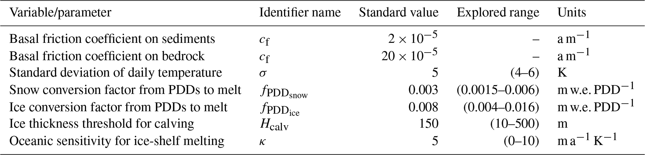
Calving takes place at the ice-shelf front when two conditions are met. First, the ice-shelf thickness must fall below a threshold Hcalv. This is a semiempirical parameter reflecting the fact that this is the typical thickness of ice-shelf fronts currently observed in Antarctica (Griggs and Bamber, 2011). Second, the upstream advection must fail to maintain the ice thickness above this threshold following a semi-Lagrangian approach (Peyaud et al., 2007) to account for the fact that ice-flux divergence fosters the formation of crevasses (Levermann et al., 2012). This method is standard in the GRISLI model. It was introduced after recognizing that a systematic cutoff of ice shelves below a given threshold led to a realistic simulation of the present-day ice shelves in Antarctica, as is the case in many models, but prevents any development of new ice shelves (Peyaud, 2006; Peyaud et al., 2007). When focusing on past climates, ice sheets should be able to evolve in response to climate changes, and in particular to allow the advance of ice shelves in cold climates. To this end, before calving ice in a certain point, we test whether advection allows for the growth of ice at the front, and therefore the ice-shelf advance. Hcalv was set to 150 m, in the standard setup. To assess the sensitivity of the ice dynamics to the value of the thickness threshold Hcalv (below which the ice is calved) we performed a new ensemble exploring a wide value range of this parameter's values, from 10 to 800 m (Fig. S4 in the Supplement). Values of this threshold above 400 m produce a drastic disintegration of the Barents–Kara complex due to its relative shallow bed. The overall effect of this sensitivity test around the preferred value is to modulate the amplitude of the response to the oceanic perturbations. Thus, GRISLI-UCM explicitly calculates grounding-line migration in addition to ice-stream and ice-shelf velocities. This allows the model to properly represent both grounded and floating ice. Note that there is no ambiguity in the model between calving and basal melt, which are two distinct processes in the model. Calving is the result of the threshold criterion described above; thus, the calving rate at a given time is given by the amount of ice lost to the ocean through this process by unit of time, converted to mass-water equivalent. Basal melt is dependent on the applied ocean temperature anomaly. GRISLI-UCM uses finite differences on a staggered Cartesian grid at a 40 km resolution, corresponding to 224×208 grid points for the Northern Hemisphere domain, including the EIS, with 21 vertical levels. By default, initial topographic conditions are provided by surface and bedrock elevations built from the ETOPO1 dataset (Amante and Eakins, 2009) and ice thickness (Bamber et al., 2001). Note there are more recent datasets for Greenland topographic features (e.g., Bamber et al., 2013; Morlighem et al., 2014, 2017). However, as Greenland is not the focus of our study, this does not affect our results. The glacial isostatic adjustment (GIA) is described by the elastic lithosphere–relaxed asthenosphere method (Le Meur and Huybrechts, 1996), for which the viscous asthenosphere responds to the ice load with a characteristic relaxation time for the lithosphere of 3000 years. For the sake of simplicity, in this study the isostatic adjustment is assumed to be only due to local ice mass variations, as other such research has assumed in the past (e.g., Greve and Blatter, 2009; Helsen et al., 2013; Huybrechts, 2002; Langebroek and Nisancioglu, 2016; Stone et al., 2010). The surface mass balance (SMB) is given by the sum of accumulation and ablation, both of which are calculated from monthly surface air temperatures (SATs) and monthly total precipitation. Accumulation is calculated by assuming that the fraction of solid precipitation is proportional to the fraction of the year with mean daily temperature below 2 ∘C. The daily temperature is computed from monthly SATs assuming that the annual temperature cycle follows a cosine function. Ablation is calculated using the positive-degree-day (PDD) method (Reeh, 1989). Its main parameters are the standard deviation of daily temperature, σ, and the conversion factors from PDDs to melt for snow and ice, and . Here, σ=5 K, m.w.e. PDD−1 and m.w.e. PDD−1. m.w.e. PDD−1. Refreezing is considered, with a value of Csi=60 % (see Sect. 2 in the Supplement). This melting scheme is admittedly too simple for fully transient paleo-simulations, as it omits the contribution of insolation-induced effects on surface melting (Robinson and Goelzer, 2014). Nevertheless, insolation changes are most relevant in long-term simulations including variations at orbital timescales, especially in past warmer periods such as the Eemian. As this study focuses on abrupt climate changes within a fixed glacial background climate, insolation changes are not important and the PDD melt model should be sufficient to give a good approximation of surface melt in response to interstadials in a reasonable manner. GRISLI-UCM accounts for changes in elevation at each time step considering a linear atmospheric vertical profile for temperature with different lapse rates in summer and in the annual mean (0.0065 and 0.0080 K m−1, respectively) to account for the smaller summer atmospheric vertical stability.
Basal melting for grounded ice depends on pressure and water content at the base of the ice sheet (Ritz et al., 2001) as well as on the geothermal heat flux, which is prescribed from the reconstruction by Shapiro and Ritzwoller (2004). Basal melting for floating ice is computed using a linear temperature anomaly with respect to the freezing point. The details of the implementation of the boundary conditions (SMB and oceanic basal melting) in this particular study are given below (Sect. 2.2). Finally, ice flow was calculated with a 1-year time step, whereas thermodynamics and boundary conditions (including PDD) were updated every 5 years. The model parameters and the range of their values explored here are shown in Table 1.
Table 1Model parameters used in this study with their standard and explored values.
2.2 Off-line forcing method
SMB and oceanic basal melting are obtained through a time-varying synthetic climatology built with a novel method that is found to provide a more realistic off-line forcing for ice-sheet models than classical off-line methods (Banderas et al., 2018). The method follows a perturbative approach in the sense that the forcing combines the present-day climatology, obtained from observational data, and simulated anomalies. However, in contrast to usual off-line forcing methods, orbital- and millennial-scale variabilities are not lumped in a sole anomaly pattern but differentiated. Thus, the method combines present-day observations, simulated LGM anomalies relative to present, scaled by an orbital-timescale index, and simulated stadial–interstadial anomalies, scaled by a millennial-timescale index:
Here, Tatm(t) and P(t) are the SAT and precipitation fields at time t. and P0 are the ERA-Interim present-day SAT and precipitation climatologies (Dee et al., 2011). and are the orbital temperature anomaly and precipitation ratio relative to the present day (not shown, see Banderas et al., 2018), respectively, obtained from previous equilibrium simulations for the preindustrial and LGM climates performed with the CLIMBER-3α model (Montoya and Levermann, 2008). and are the millennial temperature anomaly and precipitation ratio, respectively, for the interstadial relative to the stadial state (Sect. 2.3). The key differences between these climate modes as simulated by Montoya and Levermann (2008) with the CLIMBER-3α model are that in the stadial, North Atlantic Deep Water (NADW) formation is relatively weak and takes place south of Iceland. Accordingly the sea-ice front in the North Atlantic reaches 40∘ N. In the interstadial state there is a northward shift and intensification of NADW formation. Northward oceanic heat transport increases, and the North Atlantic and surrounding areas warm relative to the stadial state, in particular the Nordic seas. Thus, the simulated interstadial state is characterized by a more vigorous NADW formation and Atlantic meridional overturning circulation (AMOC) along with reduced sea ice in the Nordic seas, and a temperature increase of up to 10 K in the North Atlantic relative to the stadial state, with a maximum anomaly in the Nordic seas. Note that bold symbols indicate two-dimensional spatial fields. The stadial mode in our study is represented by a climate simulation of the LGM with CLIMBER-3α (Montoya and Levermann, 2008). The interstadial mode is taken from a recent glacial transient simulation performed with the same model under glacial climatic conditions, but with intensified NADW formation (Banderas et al., 2015). α⋆ and β⋆ are two indices that separately modulate the contribution of the orbital and millennial anomalies. Both were built based on two recent complementary temperature reconstructions over Greenland, one from the NGRIP ice-core record for the LGP (Kindler et al., 2014), and the other from several ice-core records for the Holocene (Vinther et al., 2009). Their combination (hereafter, the KV reconstruction) results in a continuous temperature reconstruction for Greenland for the past 120 kyr (Banderas et al., 2018). α⋆ is obtained after applying a low-pass frequency filter ( ka−1) to the original KV reconstruction based on a spectral decomposition; β⋆ is obtained following a similar procedure but retaining the high-frequency signal. Both indices are tuned in such a way that the resulting synthetic temperature time series at the NGRIP site exactly matches the KV reconstruction (this distinguishes α⋆ and β⋆ from the raw α and β indices previous to this tuning; Banderas et al., 2018).
The net basal melting rate for floating ice, B, is assumed to follow a linear relation:
where Tocn is the oceanic temperature close to the grounding line, Tf is the temperature at the ice base, which is assumed to be at the freezing point, and κ is the heat flux exchange coefficient between ocean water and ice at the ice–ocean interface; its standard value in the present study is κ=5 m a−1 K−1. Several marine-shelf basal melting parameterizations can be found in the literature, as recently reviewed by Asay-Davis et al. (2017). The submarine melt rate is thought to be directly influenced by the oceanic temperature variations below the ice shelves. Accordingly, most basal melting parameterizations are built as a function of the difference between the oceanic temperature at the ice-–ocean boundary layer and the temperature at the ice-shelf base, generally assumed to be at the freezing point. The dependence on this temperature difference can be linear (Beckmann and Goosse, 2003) or quadratic (Holland et al., 2008; Pollard and DeConto, 2012; DeConto and Pollard, 2016; Pattyn, 2017). The linear marine-shelf basal melting parameterization used in this study is the simplest case that allows for testing of the ice-sheet sensitivity to past oceanic temperature changes. Nevertheless, it accounts separately for basal melting below the ice shelves (away from the grounding line) and at the grounding line. The basal melting rate of the ice shelves (Bsh) is given by the grounding-line basal melt (Bgl) scaled by a constant factor (γ):
In this study, γ is set to 0.1. Thus, we consider that the submarine melting rate for ice shelves is 10 times lower than that close to the grounding zone, which is in qualitative agreement with observations in some Greenland glaciers with floating tongues (Münchow et al., 2014; Wilson et al., 2017) as well as in Antarctic ice shelves (Rignot and Jacobs, 2002; Marsh et al., 2016). Note that this value is subject to uncertainty. Although we did not explore any other values different from γ=0.1, we did consider a range of κ values between 1 and 10 m a−1 K−1, which accounts for a wide range of oceanic sensitivities (see Sect. 2.3).
As in Peyaud et al. (2007), in regions with ocean depths above 750 m, an artificially large melting rate (20 m a−1 is prescribed to avoid unrealistic growth of ice shelves beyond the continental-shelf break, where they would likely be subject to high melt rates in reality because of high heat exchanges with the ocean.
Following the approach described above, Tocn(t) is assumed to be given by an expression analogous to Eq. (4). Thus Eq. (6) can be rewritten as follows:
where represents the present-day oceanic basal melting rate.
Finally, millennial-scale sea-level variations are prescribed according to the reconstruction by Grant et al. (2012, Sect. 2.3). The specific details of the experimental setup used are described below.
2.3 Experimental setup
In this study, we investigate the response of the EIS to millennial-scale climate variability during MIS 3. The starting point of our experiments is a control-run ice-sheet simulation with constant boundary conditions for MIS 3 that provides a representative configuration of the EIS for that time period (Fig. 1). To this end, α⋆ was set to its value at 40 ka BP, that is, , and to preclude millennial-scale variations. Note, however, that these values are to a certain extent arbitrary; they are intended to provide a stable mean background state similar but not necessarily identical to background MIS 3 conditions. Thus,
Note that although Eq. (11) is formally correct and consistent with the scheme used, in contrast to the present-day SAT or precipitation the present-day rate of oceanic basal melting cannot be determined. Thus, in practice we replace this equation by directly tuning the value of B40 K to obtain a reasonable ice-sheet configuration at 40 kyr BP (Fig. 2) given the atmospheric forcing fields expressed by Eqs. (9)–(10). To this end, a constant basal melting rate of 0.1 m a−1 is assumed. The ice sheet was forced with the resulting climatologies for 100 kyr previous to the start of the perturbations described below. This allows the vertical temperature profile within the ice sheet to be equilibrated with the climate. This procedure was found to facilitate the growth of European ice sheets within the reconstructed limits for 60 and 20 kyr BP (Svendsen et al., 2004; Kleman et al., 2013) (Fig. 2).
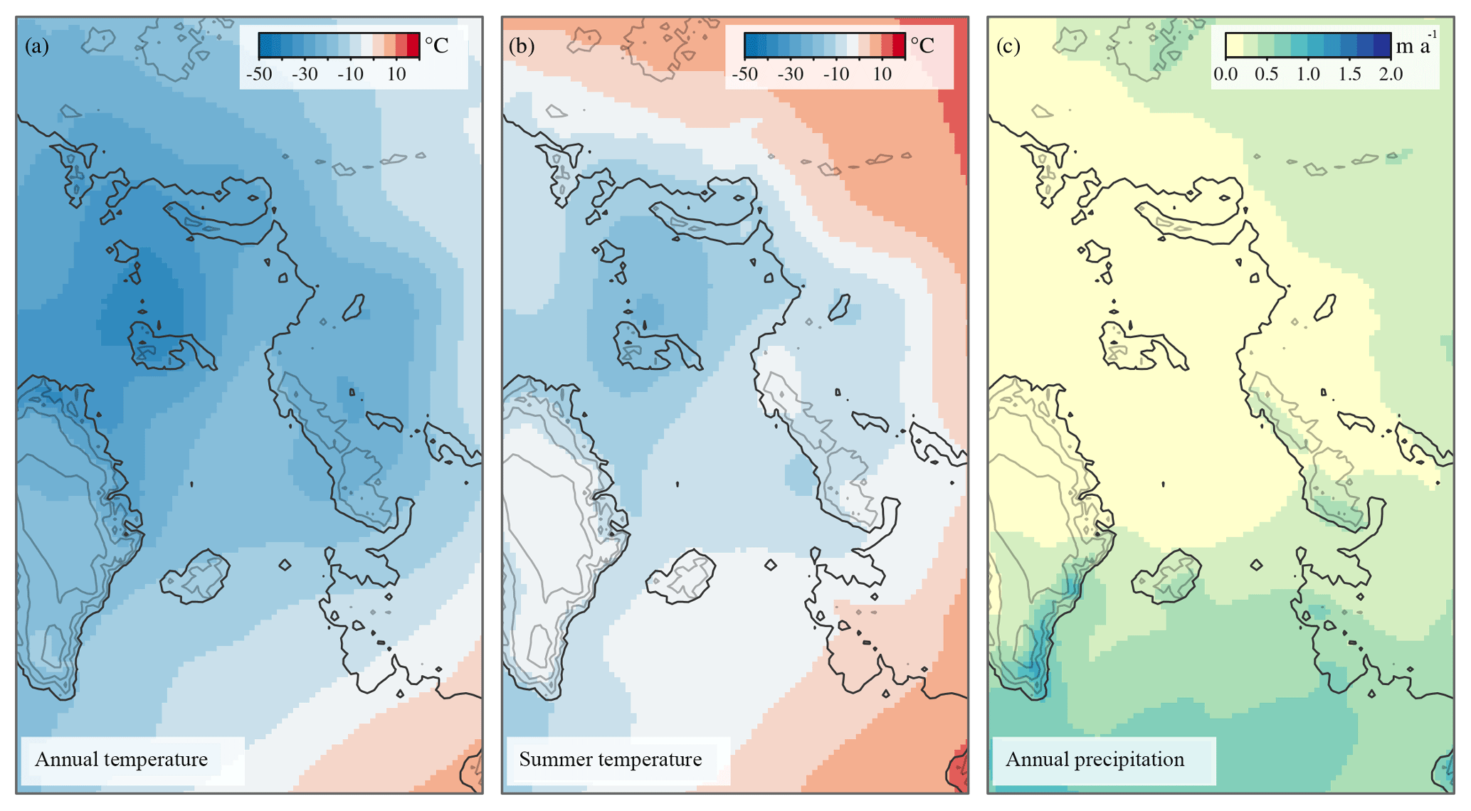
Figure 1Background climatic forcing for the control run (CTRL). MIS 3 (∼40 kyr BP) reference annual mean SAT (a) and summer mean SAT (b) in degrees Celsius and annual mean precipitation in meters per annum (c). Present-day contour lines with the land boundary delineated at a depth of −80 m are added for reference.

Figure 2Resulting ice sheet of the MIS 3 control run (CTRL). Simulated ice thickness with contours plotted for every 500 m. The grounding-line position is shown using a black line, the 500 m depth contour is shown using a white line and velocities are shown using the shaded colors (in kilometers per annum) after the spin-up was completed. This ice sheet represents the initial state previous to the application of perturbations. Bjørnøyrenna Basin, as referenced in the text, is shown using the black rectangle. The Barents–Kara, Scandinavian and British Islands regions are highlighted using blue, red and purple rectangles, respectively.
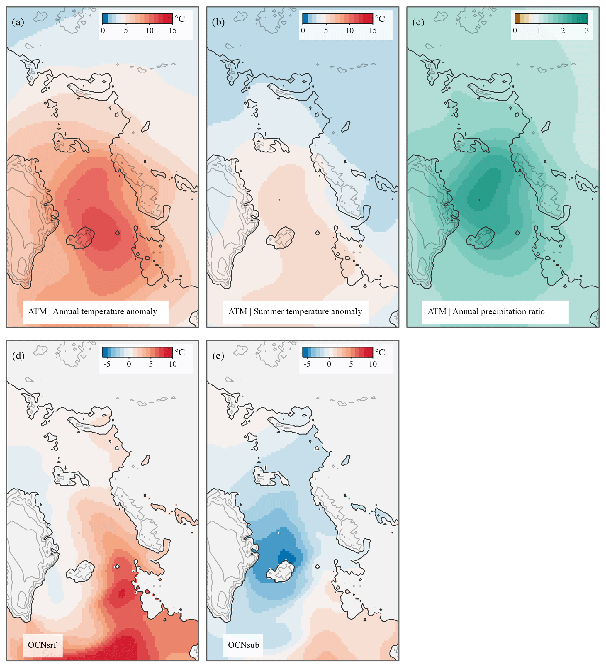
Figure 3Millennial-scale components of the boundary forcing. (a) SAT anomalies (interstadial minus stadial) in degrees Celsius. (b) Summer SAT anomalies (interstadial minus stadial) in degrees Celsius. (c) Precipitation ratio (interstadial to stadial). (d) Anomalies of SST and (e) subsurface ocean temperature (at a depth of 500 m) in degrees Celsius. Present-day contour lines with the land boundary delineated at a depth of −80 m are added for reference. Note that to force the ice-sheet model these fields are scaled to reproduce the NGRIP interstadial minus stadial temperature change.
Our forcing method allows for the response of the EIS solely to millennial-scale climate variability at MIS 3 to be investigated by keeping the orbital component of the forcing () constant and letting β⋆ vary throughout the LGP (Eqs. 4, 5, 8). In order to assess the relative roles of the atmosphere and the ocean, three independent experiments are carried out. First, an atmospheric-only forced simulation (ATM) in which the time evolution of SAT and precipitation on millennial timescales is considered, while the oceanic forcing is kept constant with MIS 3 (i.e., 40 kyr BP) background climatic conditions. Thus,
Second, an oceanic-only forced simulation (OCN) in which the atmospheric forcing is kept constant, while the oceanic basal melting is allowed to vary at millennial timescales around its background MIS 3 value:
The magnitude and sign of oceanic temperature anomalies ΔTocn depends on the depth at which Tocn is considered. In our simulations, a large part of the northeastern sector of the EIS is marine based with shallow bedrock depths between 500 m and less than 100 m in several locations further south. Therefore, it is unclear whether this marine ice sheet should be more susceptible to changes in the surface or the subsurface of the ocean.
To investigate the effect of this uncertainty, we decided to perform two different simulations considering different depths: one corresponding to the surface (OCNsrf) and the other considering deeper (subsurface) oceanic waters by averaging temperatures within the depth range of 400–600 m (OCNsub). Therefore we hereafter distinguish between for surface or subsurface millennial-scale temperature anomalies, respectively (Fig. 3). The realism and convenience of applying one or the other is addressed in Sect. 4.
Finally, a simulation “ALL” was carried out combining both the atmospheric and the oceanic forcings:
In all experiments β⋆(t) dictates the millennial-scale variability of the forcings (Fig. 4a). Because our simulated stadial–interstadial transition results from an intensification of the AMOC, positive β⋆ values imply an increase in Tatm relative to its background MIS 3 value (e.g., Eq. 18; Figs. 3, 4). As a consequence, the atmosphere warms at interstadials relative to stadial periods, as reflected by the millennial-scale anomaly field (Fig. 3a, b). Note that refreezing is not allowed to occur in our current model setup. If (which would imply B(t)<0), we simply impose the value B(t)=0.
Table 2Millennial-scale components used to force the ice-sheet model in the different experiments shown in this study.
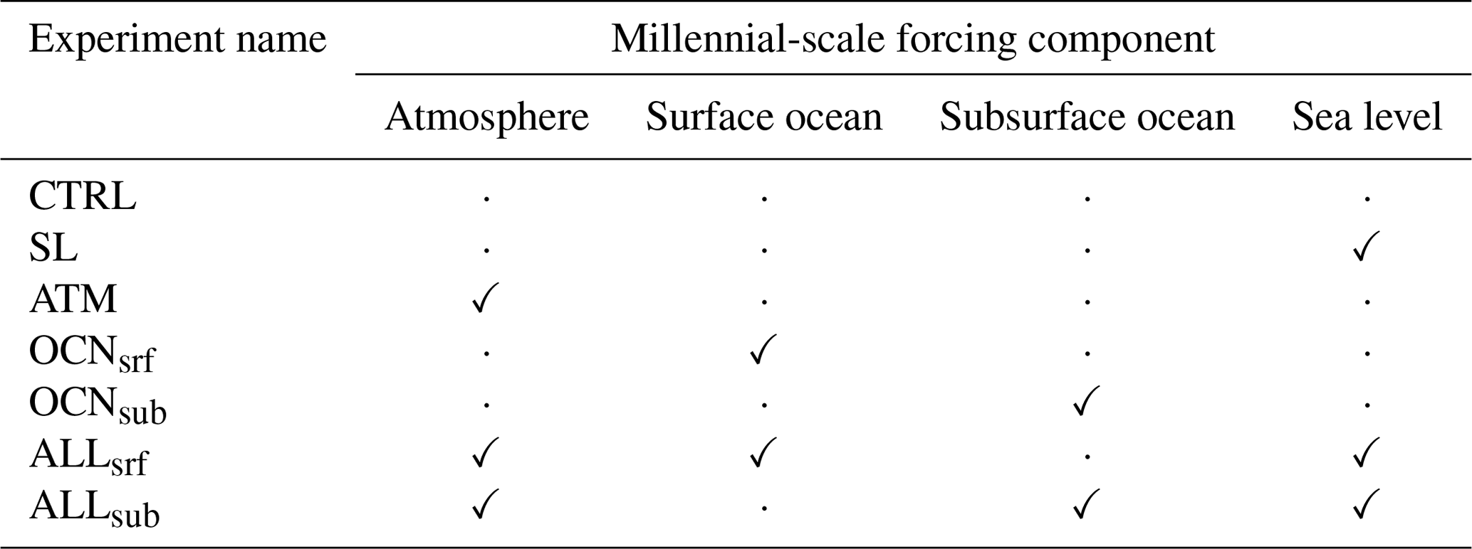

Figure 4(a) Temporal component of the millennial-scale climatic forcing (β⋆ index). (b) Millennial-scale sea-level forcing (Grant et al., 2012). (c) EIS sea-level equivalent (in meters) related to ice volume variations (in cubic meters) with respect to initial conditions for the CTRL run (black) and for the SL (gray), ATM (gold), OCNsrf (blue), OCNsub (red), ALLsrf (dark blue) and ALLsub (dark red) forcing experiments.
An ensemble of simulations for different values of κ have been considered to evaluate the sensitivity of the EIS to the forcing. Finally, varying sea-level forcing is considered (Fig. 4b), both alone (SL) and in combination with the previous forcings (ALL).
We analyze the response in terms of the ice volume evolution, the mass balance and the grounding-line dynamics. The different simulations analyzed here are summarized in Table 2.
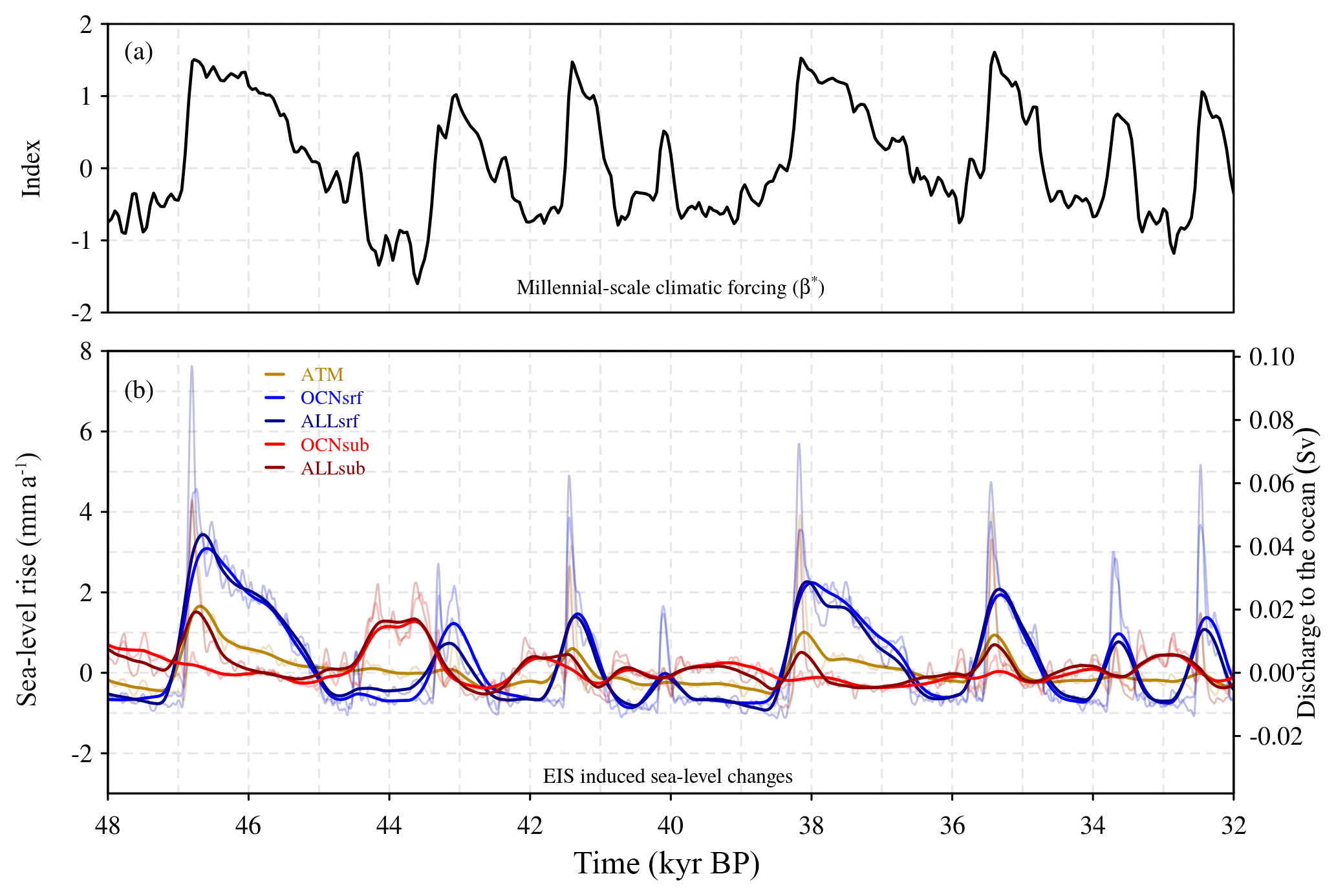
Figure 5MIS 3 period. (a) Temporal component of the millennial-scale climatic forcing (β⋆ index), and (b) EIS changes (in millimeters per annum and Sv) related to ice volume variations with respect to initial conditions for the CTRL run (black) and for the SL (gray) ATM (gold), OCNsrf (blue), OCNsub (red), ALLsrf (dark blue) and ALLsub (dark red) forcing experiments. Thick lines show the variables after applying a low-pass filter of 100 years.
3.1 Ice volume evolution
Substantial differences are found in the response of the EIS to the forcing scenarios. Under constant forcing, the CTRL run shows negligible millennial-scale sea-level equivalent (SLE) variations, although a lower frequency SLE fluctuation is found as a result of internal ice-sheet variability (Fig. 4) through a thermomechanical feedback. This slow variability appears only in the southernmost parts of the Eurasian ice sheet where ablation exists. It is due to an interplay between the available basal water favoring sliding and the EIS associated thinning due to an increase in velocities. As this phenomenon concerns only the ablative borders of the ice sheet and its frequency corresponds to more than 20 kyr, its governing dynamics is not detailed here. When the model is forced only by changes in sea level (SL run), a small response of approximately 0.5 m SLE is observed on millennial scales. These changes appear not to be sufficient to cause a substantial migration of the grounding line, and thus do not affect ice velocities (not shown). In ATM, the atmospheric forcing alone causes a sequence of enhanced ablation episodes resulting in modest ice volume variations (up to 1.5 m SLE) during the most prominent stadial–interstadial transitions; this represents a change of approximately 7 % with respect to the initial ice-sheet volume. In contrast, the oceanic forcing in OCNsrf induces pronounced changes in the dynamics of the EIS on millennial timescales (see below), with episodes of large volume reduction occurring during interstadials. The combination of sea level, atmospheric and oceanic forcings (ALLsrf) results in a very similar response of the EIS to that obtained in OCNsrf (Fig. 4) as a consequence of the larger effect of the oceanic forcing in OCNsrf with respect to ATM. OCNsub shows an antiphase relationship with respect to OCNsrf, with the largest reductions in ice volume occurring during prolonged stadial periods and regrowth during interstadials. This behavior can be explained by the fact that ocean waters at the subsurface warm (cool) during episodes of reduced (enhanced) convection in the Nordic seas as a result of variations in the AMOC strength (Fig. 3d, e). Note that the antiphase relationship is, however, not perfect. At the surface, the largest anomalies are found off the North Atlantic, the British Isles and the Norwegian coast, and result from the intensification of Atlantic northward heat transport associated to the enhanced AMOC during interstadials; at the subsurface the concomitant cooling is largest in the Nordic seas as a result of enhanced heat loss to the atmosphere associated with enhanced convection.
Thus, the out-of-phase relationship found in the dynamic response of the EIS between these two oceanic experiments results from the opposed sign of their spatial forcing patterns (Fig. 3). When considering the forcing at the subsurface of the ocean along with the atmosphere (ALLsub), slight reductions of the EIS volume (less than 1 m of SLE) during interstadials are superimposed onto the previous behavior (Fig. 4).
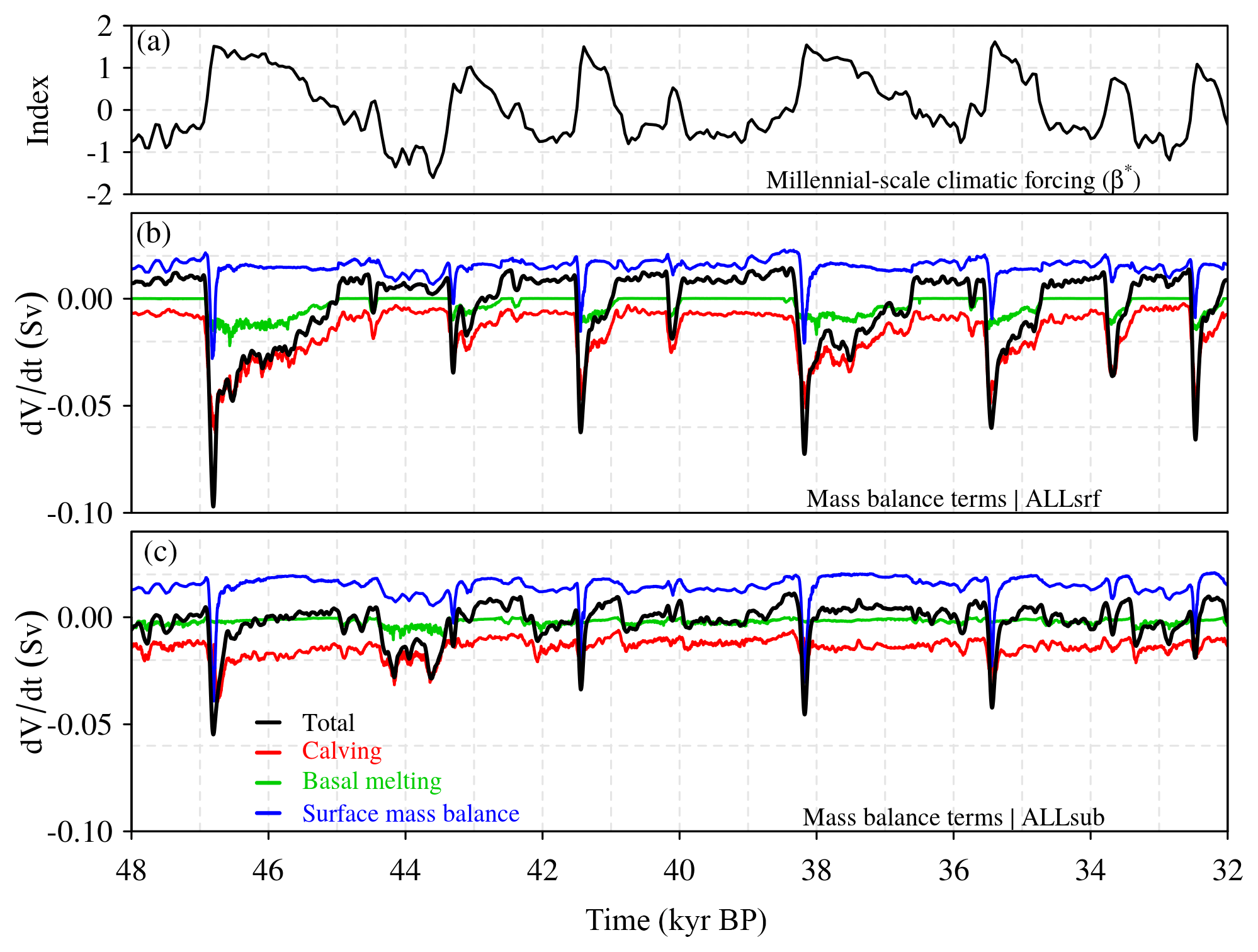
Figure 6MIS 3 period. (a) Temporal component of the millennial-scale climatic forcing (β⋆ index), and the contribution of the different terms of the EIS mass balance to ice volume variations (Sv) in the simulations considering all forcings, with (b) corresponding to the surface oceanic forcing (ALLsrf) and (c) to the subsurface oceanic forcing (ALLsub). The calving and basal melt rates are given by the amount of ice lost to the ocean through the calving and basal melting parameterization per unit of time, converted to water-equivalent volume.
As a consequence of the millennial-scale forcing, a trend in ice volume from its initial value of 8.3×10¹⁵ km3 (about 21 m SLE) leading to a loss of 8–12 m SLE is found. This is a consequence of the fact that no refreezing is allowed and that a positive constant (and spatially uniform) basal melting of 0.1 m a−1 was imposed. As a consequence, accumulation is not able to compensate for ice loss through basal melt and calving after each ice-mass loss event. Note, however, that background conditions are fixed at 40 kyr BP; in a more realistic setup, as time proceeds forward, orbital forcing leading to gradually colder conditions would be expected to aid in the ice regrowth, thereby helping with its growth throughout the LGP. Spatially nonuniform background melting is also conceivable. However, we have no information on what this background value would have been. Because our focus was the response of the EIS to millennial-scale climatic variability, we opted for the simplest experimental setup possible, meaning a spatially uniform and fixed-in-time background value perturbed by a millennial-scale index.
The magnitude of these changes in terms of sea-level rise rate and discharge, specifically for the MIS 3 period, is illustrated in Fig. 5. The simulations forced with the surface of the ocean (OCNsrf and ALLsrf) show the largest amplitudes, with peaks of sea-level rise above 4 mm a−1 during DO-events and sustained contributions well above 1 mm a−1 during entire interstadial periods. In ATM, a decline of the EIS during stadial–interstadial transitions is still observed but presents a smaller amplitude of 1–2 mm a−1. The simulations in which the ice sheet is forced with the subsurface of the ocean (OCNsub and ALLsub) present a decline of their volume during stadial periods and regrowth during interstadials as a consequence of the inverted spatial pattern of temperature anomalies with respect to the surface. In OCNsub (and ALLsub) the amplitude of these changes is smaller than in OCNsrf (and ALLsrf), in the order of 0.5–1 mm a−1, reaching more than 1 mm a−1 during pronounced stadials (as ca. at 44 kyr BP). The ALLsrf and ALLsub simulations show a similar or slightly larger volume loss during interstadials, as a consequence of the additional atmospheric forcing, which is superimposed onto the OCNsrf and OCNsub behavior.
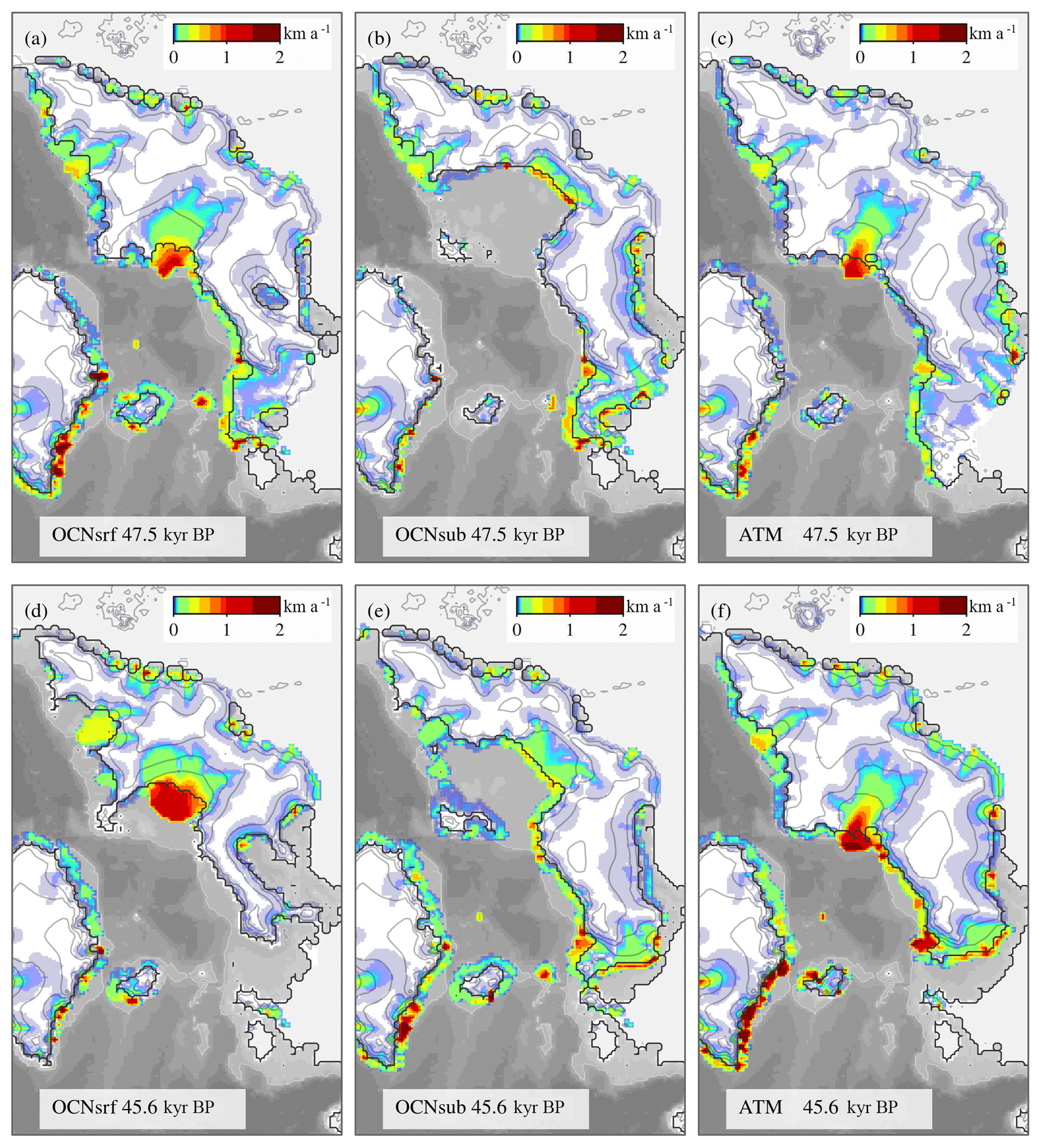
Figure 7Simulated EIS at the end of a stadial period (a–c) and at the end of an interstadial period (d–f) for the OCNsrf (a, d), OCNsub (b, e) and ATM (c, f) experiments. Shaded colors show ice velocities (in kilometers per annum). The ice thickness contours are plotted for every 500 m with the grounding-line position shown using a black line. The 500 m depth contour is shown using a white line. The periods represented here corresponds to the stadial and interstadial periods prior and posterior to DO 12 (ca. 47 kyr BP), respectively.
3.2 Mass-balance response
The response of the EIS has been analyzed in terms of its mass balance decomposition for the all-forcing runs (Fig. 6). In ALLsrf the surface ocean temperature varies in phase with the atmosphere (Fig. 3). Thus, during stadial–interstadial transitions, the high negative values of dV/dt can be explained by the conjunction of an initial sharp increase in ablation and pronounced increases in basal melting and calving, which allow for a large grounding-line retreat in the Bjørnøyrenna Basin (Fig. 6b). The rate of ice loss by basal melting is similar to that resulting from the increase in ablation (as reflected in the SMB) during the peak of a stadial–interstadial period. However, basal melting is much more efficient than surface mass balance at decreasing volume along the whole duration of an interstadial. This is due to the fact that ablation is restricted to the southern borders of the EIS. Thus, when the ice sheet has retreated to areas of no ablation, in spite of a slight further loss provided by the elevation feedback, it rapidly equilibrates and a negative surface mass balance cannot propagate further inland. In contrast, when enhanced basal melting from higher oceanic temperatures is applied, the associated retreat can propagate further inland occupying a large proportion of the Bjørnøyrenna Basin and facilitating high rates of volume loss (although similar in amplitude with respect to SMB) during the whole interstadial period (see the animation corresponding to ALLsrf and Fig. S5 in the Supplement). Note that basal melting, together with calving, is a very efficient method to remove ice; basal melting leads to thinning of the ice shelf which can subsequently undergo calving. During stadial periods, both the enhanced positive mass balance and the absence of basal melting (favored by the negative oceanic anomalies) favor the regrowth of the EIS. Subsurface ocean temperatures also evolve in phase with the atmosphere in the southwestern part of the EIS but in antiphase in its northeastern part. In other words, when forcing with the subsurface of the ocean, a slight warming (cooling) is observed around the Britain–Ireland ice sheet while cooling (warming) of the Bjørnøyrenna Basin is simulated during interstadial (stadial) periods (see Fig. 3). Therefore, the ALLsub simulation presents volume declines during stadial–interstadial transitions due to an increase in ablation and basal melting in the southwestern part. The corresponding mass fluxes reach up to about 0.05 Sv; of these, approximately 0.025, 0.02 and 0.005 Sv originate in the Barents–Kara, Scandinavia and the British Islands, respectively. Subsequently, reduced basal melting in the northeastern part of the EIS favors regrowth of the Bjørnøyrenna Basin during interstadial periods. Finally, shifting to pronounced stadial periods (as in ca. 44 kyr BP) favors the penetration of warm subsurface waters that increase basal melting enough to produce an ice-sheet retreat in the northeastern part in spite of the enhanced positive surface mass balance (Figs. 5, 6). When considering the atmosphere and the subsurface ocean forcing together in ALLsub, these competing processes translate into a smaller amplitude of millennial-scale EIS changes compared with the case with surface ocean forcing (ALLsrf). Furthermore, declines of the EIS can be observed both during the beginning of interstadial periods and during pronounced stadial periods in ALLsub (Figs. 5, 6).
Focusing on the OCN and ATM simulations separately facilitates isolating the effects of the ocean on this complex pattern. To this end, the simulated ice-sheet distribution and velocities of OCNsrf, OCNsub and ATM are shown in Fig. 7 for the period around DO-event 12, at ca. 47 kyr BP. As expected, OCNsrf shows a widespread retreat both in the northeast and the southwest of the EIS from the stadial to the interstadial period (Fig. 7d). This is accompanied by an acceleration of the Bjørnøyrenna Basin due to its grounding-line thinning and retreat (Fig. 7a, d). OCNsub presents a collapsed Bjørnøyrenna Basin during the stadial period previous to DO-event 12 due to enhanced basal melting from warmer subsurface waters. The transition to the interstadial period favors a slight regrowth of this northeastern part of the EIS due to decreased basal melting, while its southwestern section slightly retreats (Fig. 7b, c)
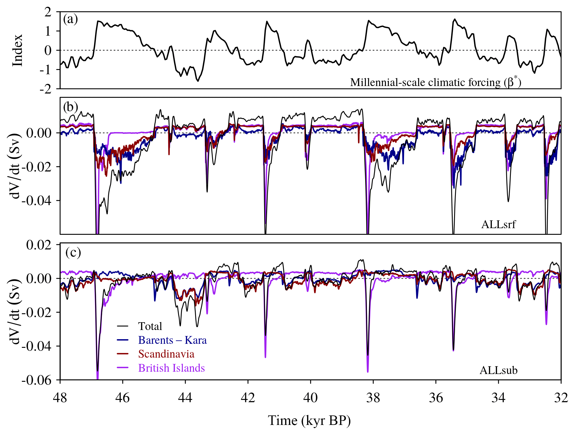
Figure 8MIS 3 period. (a) Temporal component of the millennial-scale climatic forcing (β⋆ index), and the contribution of the different regions to ice volume variations (Sv) in the simulations considering all forcings, with (b) corresponding to the surface oceanic forcing (ALLsrf) and (c) to the subsurface oceanic forcing (ALLsub). The geographical domains of the different regions are highlighted in Fig. 2.
Concerning ATM, only in the southwestern part of the EIS is the atmospheric forcing capable of generating an important reduction in the EIS volume in response to the stadial–interstadial transition (Figs. 7c, f, S5). This is a result of the spatial pattern of the forcing, with the largest SAT anomalies located around the Nordic seas (Fig. 3). Therefore, the ice volume reduction of the EIS in ATM during interstadials is due to the positive SAT anomaly, which leads to enhanced ablation in the southwestern part of the EIS (Fig. S5). In turn, reduced SATs during stadials allow the regrowth of the ice sheet up to the continental margin of the Nordic seas. The more active dynamic response of the EIS in the OCN simulations can be attributed to the increase in oceanic temperatures by 2–4 ∘C (Fig. 3) within the margins of the ice sheet during interstadial (in the case of OCNsrf) and stadial (OCNsub case) periods, which translates into enhanced basal melting at the margins of the EIS. The southwestern sector of the EIS also responds to the warmer SSTs, even displaying a larger reduction of ice volume than in ATM (Fig. 7).
The spatial patterns shown in Fig. 7 are representative of the ice-sheet response during all other stadial–interstadial transitions. In OCNsrf, the EIS reacts to every abrupt surface warming with a substantial ice-flow acceleration, especially in the Bjørnøyrenna Basin (Figs. 7, 8, 9). Ice shelves that are present during stadial periods suddenly retreat during DO-events and in combination with enhanced basal melting favor thinning and retreat of the grounding line that translate into large iceberg discharges of up to ca. 0.06 Sv. In OCNsub, ice velocities in the Bjørnøyrenna Basin increase during stadials, when enhanced basal melting erodes the grounding line and favors its retreat. Peaks in calving are recorded accordingly during pronounced stadial periods (Fig. 10). However, these peaks are of smaller amplitude than in OCNsrf. This can be explained by the fact that, along the coast of Eurasia, the amplitude of the simulated SST anomalies used to compute basal melting in OCNsrf is larger than the subsurface temperature anomalies in OCNsub, as the basal melt was calculated by using ocean temperature at a fixed depth, either at the surface or at the subsurface. Also, transitions to stadials are usually more gradual than transitions to interstadials; thus, in this case, the incursion of warmer (subsurface) waters occurs in a smoother manner. High velocities reach their maxima at the end of the stadial and beginning of the interstadials. However, the latter are not accompanied by an increase in calving due to the fact that ice shelves are expanding and thickening during this period thanks to reduced basal melting (Fig. 10). In general, the extension of ice shelves is greatly reduced during periods of enhanced basal melting (Figs. 9, 10), with no large unconfined ice shelves surviving during these episodes. Some thinner ice shelves remain, in spite of the enhanced basal melting, thanks to an increase in advection from the Bjørnøyrenna ice stream triggered by a grounding-line retreat (Fig. 7).
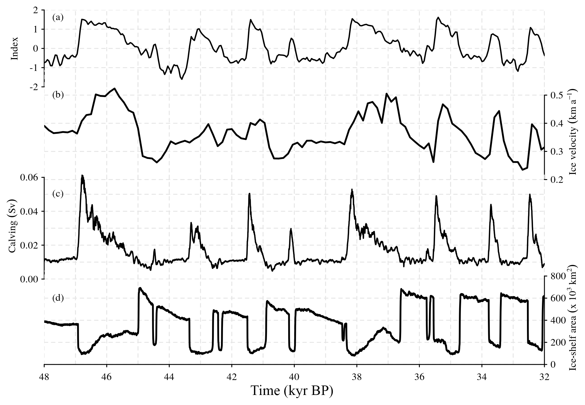
Figure 9MIS 3 period. Temporal component of the millennial-scale climatic forcing (β⋆ index), ice velocities in the Bjørnøyrenna Basin (calculated as mean values over the entire basin in kilometers per annum), calving rate (Sv) and ice-shelf area (103 km2) in the OCNsrf simulation.
3.3 Grounding-line dynamics
Changes in the position of the calving front are usually accompanied by a grounding-line displacement (not shown). For some minor ice-shelf breakups this close relationship can be broken, but with almost no effects upstream inland. Thus, we consider that the grounding-line position is the best indicator for characterizing the dynamic behavior of the marine part of the EIS. Inspection of the temporal evolution of the grounding-line position in OCN simulations confirms that ice dynamics control the majority of ice-volume variations in the EIS as opposed to the SMB processes involved in ATM (Fig. 11). The migration of the grounding line through time has been characterized by means of an index (μ) that weighs the proportion of non-grounded points in the region of the Bjørnøyrenna Basin:
where Ng(t) represents the evolution of the number of points of grounded ice within a fixed area of N points in the Barents Sea region defined over the black square highlighting the Bjørnøyrenna Basin shown in Fig. 2. Note that other metrics are also possible; the same metric has been used in other studies in different domains such as Antarctica (Blasco et al., 2018).
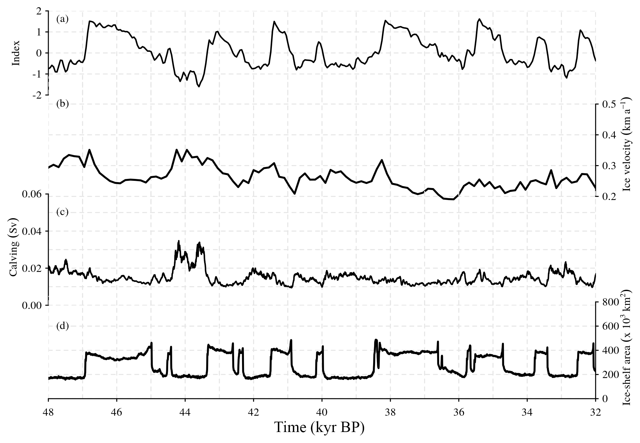
Figure 10MIS 3 period. Temporal component of the millennial-scale climatic forcing (β⋆ index), ice velocities in the Bjørnøyrenna Basin (calculated as mean values over the entire basin in kilometers per annum), calving rate (Sv) and ice-shelf area (103 km2) in the OCNsub simulation.
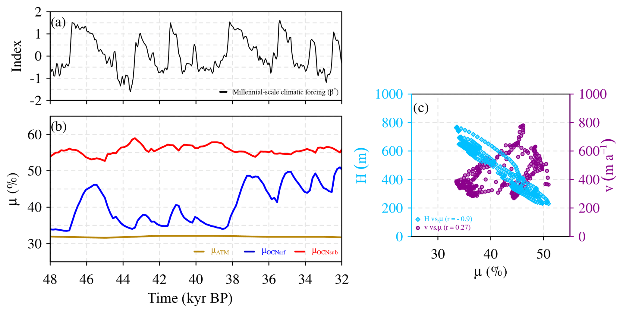
Figure 11Dynamic behavior of the EIS during millennial-scale climatic transitions for the OCNsrf, OCNsub and ATM experiments. Displacement of the grounding line in the Bjørnøyrenna Basin (b) in response to the climatic β⋆ forcing (a). The evolution of the grounding-line position is shown for OCNsrf (blue), OCNsub (red) and ATM (gold). The migration of the grounding line has been characterized as an index μ(t) that represents the evolution of the number of points of grounded ice Ng(t) over a fixed area of N points in the Barents Sea region, defined over the black square highlighting the Bjørnøyrenna Basin shown in Fig. 2. Increasing values of μ indicate grounding-line retreat. (b) OCNsrf scatterplot diagram showing the relationship between mean ice thickness H in the region of the Bjørnøyrenna Basin and μ (light blue diamonds) as well as the relationship between ice-stream velocities v in the same region and μ (purple circles).
Thus, an increase (decrease) in μ indicates a retreat (advance) of the grounding line. While in ATM μ barely changes Fig. 11), OCN runs show a large dynamic behavior of the basin. In OCNsrf, μ reflects a synchronous evolution of the grounding-line position and the oceanic forcing, with major retreats coinciding with interstadial states (Fig. 11). Conversely, the Bjørnøyrenna Basin is generally much closer to a full retreat in OCNsub during stadials due to a larger penetration of warm subsurface waters (Fig. 3; OCNsub) compared to the surface waters (Fig. 3; OCNsrf). However, the grounding line is able to advance and reach Svalbard during episodes of reduced basal melting at the interstadials.
The direct coupling between the oceanic forcing and the response of the Bjørnøyrenna ice stream is also evident from the relatively high negative correlation () found between μ and ice thickness in this area (Fig. 11). A local thinning of the grounding line produced by a warmer ocean triggers its retreat and starts the propagation of the dynamic imbalance of the ice stream. The propagation of a change in the surface slope occurs almost instantaneously at these timescales (with a typical propagation speed of about 10 km a−1). This chain of processes explains the tightened linear relationship between the Bjørnøyrenna Basin thickness and the grounding-line position, μ. Although a grounding-line retreat (advance) of the grounding line in this region produces an acceleration (deceleration) of the ice streams, its linear relationship is less obvious than that for ice thickness (Fig. 11c). This is explained by the fact that ice-stream velocities lag the grounding-line imbalance due to the characteristic time for the kinematic wave to propagate along the ice streams of the whole basin (typically of ∼1 km a−1).
As a consequence of the destabilization of the ice sheet, important ice-volume variations observed in the northeastern part of the EIS during millennial-scale climatic transitions, which added to the minor contribution of the southwestern retreat (Fig. 8), result in fluctuations of more than 4 m SLE in OCNsrf, up to 2.5 m in OCNsub and ca. 1 m in ATM (Fig. 4).
In order to investigate the sensitivity of the results to the model parameters, eight additional OCN simulations, both for the surface and the subsurface, have been carried out with different κ parameters between 1 and 10 m a−1 K−1, i.e., bracketing our standard case of κ=5 m a−1 K−1. This choice reflects the inferences based on measurements made on Antarctic ice shelves that a variation of 1 K in the effective oceanic temperature changes the melt rate by ca. 10 m a−1 (Rignot and Jacobs, 2002; Shepherd et al., 2004). A robust response of the EIS is found, with a more reactive EIS response for increasing κ values (see Sect. S1 in the Supplement). The sensitivity of our results to the values of the atmospheric mass balance model has also been explored. In spite of largely exploring the values of the parameters that determine the sensitivity to surface mass balance, the EIS variability induced by the ocean is always found to be of greater amplitude than the one induced by the atmosphere provided that κ>2 m a−1 K−1 (see Fig. S3 of the Supplement).
Our results suggest a highly dynamic Eurasian ice sheet at millennial timescales largely responding to changes in the ocean temperatures. Some authors (e.g., Gudlaugsson et al., 2013) present the marine based Barents–Kara complex as an analogue for the present-day West Antarctic ice sheet for which bedrock topography is a major control for stability. We have shown, in this sense, that the Bjørnøyrenna Basin is highly susceptible to changes in the oceanic temperatures.
Our results indicate that the timing of the response with respect to changes registered in Greenland (i.e., their occurrence during stadials or interstadial) depends, however, on whether the surface or the subsurface of the ocean is considered as the relevant forcing of the ice sheet. Recently, IRD peaks of Fennoscandian origin reported from a high-resolution marine sediment core from the Norwegian Sea indicate the presence of more frequent IRD deposition and thus calving during interstadials than during stadials (Dokken et al., 2013). This result has been corroborated in a compilation of new and previously published data (Becker et al., 2017) clearly showing that the IRD deposition increases within interstadials within MIS 3. The coeval deposition of carbonate-rich, sorted fine sands and near-surface warming suggests the presence of Atlantic water along the margin, and is interpreted by the authors as the effects of winnowing due to an intensified AMOC during interstadials. This interpretation results in concordance with our results when considering the surface waters as the oceanic forcing. Thus, this agreement would play in favor of considering that the EIS was primarily responding to changes in the surface of the ocean along the southwest EIS (Irish/Scottish margin) at least.
An out-of-phase relationship is found in the dynamic response of the EIS when forcing the ice-sheet model with the millennial-scale simulated surface and subsurface temperature anomalies. This behavior results from the roughly opposite sign of their spatial forcing patterns in the Nordic seas. This pattern has been found to be robust in a number of models but its details could well be model dependent, and, in particular, dependent on the precise location of the convection sites affected (e.g., Brady and Otto-Bliesner, 2011; Mignot et al., 2007; Montoya and Levermann, 2008; Shaffer et al., 2004; Flückiger et al., 2006).
Our results also provide a mechanism to explain the pervasive presence of IRD in the North Atlantic during MIS 3, both during stadials and interstadials, and originating both in the LIS and the EIS. During stadials, the simultaneous appearance of IRD across the wider North Atlantic Ocean can be explained by the buildup of subsurface heat in the high-latitude North Atlantic leading to increased iceberg calving in the presence of large, thick ice shelves, and lower surface temperatures allowing for wider dispersal of icebergs (Barker et al., 2015). According to our results interstadials could lead to enhanced calving of the EIS through oceanic surface subglacial melting as a result of the warmer surface conditions and relatively shallow grounding lines of this ice sheet.
The identification of IRD layers with increased calving through ice-sheet instabilities must be taken with caution, as it is based on several untested assumptions (Clark and Pisias, 2000): (i) the delivery of IRD to a specific site is caused solely by iceberg calving, versus transport by sea ice; (ii) an increase in IRD represents an increase in the iceberg flux, versus a greater amount of debris incorporated at the base of the ice sheet that delivers the icebergs, or a greater distance of iceberg transport; (iii) the amount of IRD carried by all the icebergs is similar, therefore assuming a direct relationship between IRD concentration and iceberg flux. However, the former assumptions have not been confirmed and, thus, the calving–IRD relationship might not be so direct. In addition, ocean temperatures affect melting of icebergs and thus their release of IRD. Variations in ocean temperatures can alter the IRD released by an iceberg at a certain site, causing variations in IRD deposition even for a constant amount of icebergs produced at the source.
Given the conclusion that the ocean plays a major role in abrupt ice-sheet changes, the model's treatment of grounding-line dynamics is a key issue. Several studies have shown that for many applications, a resolution of around 1 km is needed to accurately determine the grounding-line position. Sub-grid parameterizations (e.g., Feldmann et al., 2014; Winkelmann et al., 2011) or flux adjustment derived from analytic formulations (e.g., Schoof, 2007) have been proposed as methods to treat the grounding line in coarse resolution models. In addition, it has been shown (e.g., Gladstone et al., 2017) that the grounding-line behavior is sensitive to the choice of friction law and the physics of submarine melting, and that these determine model-resolution requirements. In our case, the dependence of basal drag on effective pressure allows for the desirable property of basal drag going to zero at the grounding line. However, our basal melt parameterization does not provide a smooth transition from grounded to floating ice. Thus, our results regarding the key role of the ocean on the grounding-line position can be affected by the coarse model resolution. Computational constraints do not allow for the required high model resolution, especially with a three-dimensional finite difference model on these long timescales. However, the potential inaccuracy of the grounding-line position introduced by the coarse resolution, typically of ∼100 km (Vieli and Payne, 2005; Gladstone et al., 2017), is 1 order of magnitude smaller than the grounding-line migrations simulated here (more than 1000 km). This issue should be investigated in the future, both at much higher resolution and including different formulations of friction and submarine melting.
Furthermore, it has been suggested (Pollard et al., 2015) that the ice front can suffer dramatic calving in vertical termini glaciers due to the so-called cliff instability mechanism. This process is not parameterized in our model. We believe its inclusion would, if anything, amplify the simulated response of the EIS to the ocean forcing. Nonetheless, the necessity of including this phenomenon in ice-sheet models has recently been contested (Edwards et al., 2019).
Our experimental setup is not intended to match the paleorecord, but to provide insight into the response of the EIS to millennial-scale variability. The EIS variations simulated here represent the upper-end amplitude of potential responses during the whole glacial cycle, due to its large size. Extending the study to cover the whole LGP requires the consideration of orbital variability as part of the forcing (see the Supplement). In this case, the EIS is smaller during the mildest phase of MIS 3, thus limiting its contact with the ocean and the production of iceberg discharges (Fig. S6).
Furthermore, our results depend somewhat on the particular SAT and oceanic temperature anomaly patterns simulated by our climate model, the magnitudes of the resulting forcing, and the initial size of the simulated EIS. As the response to the ocean has been found to be dominant, a larger ice sheet, with more developed ice shelves and thus more exposed to the ocean would be prone to suffer stronger basal melting; destabilization of ice shelves could therefore result in a more dynamic ice sheet with larger calving peaks. A smaller ice sheet would consequently only be affected by atmospheric forcing. The use of different atmospheric realizations is subject to the availability of climate simulations with different models for the three climate states needed: glacial (stadial), present and interstadial. The latter is only available for a reduced number of models. This makes the assessment of this issue difficult in the present study. Assessing the sensitivity to these features should be in the scope of future work, and illustrates the need for carrying out new simulations of both the interstadial and the stadial states using more sophisticated climate models. Nonetheless, our results indicate that the ocean is the major driver of the EIS ice-volume changes during MIS 3. Note that the temporal index used is the same for the atmosphere and the ocean, and the amplitude is given by an ocean general circulation model simulation of two different oceanic states mimicking stadial and interstadial periods. We then translate those fields into ablation (via PDD, for which the uncertainty has been extensively explored) and into basal melting (using a linear equation). It is conceivable that our synthetic oceanic temperature forcing is larger than that deduced from reconstructions in certain locations, which range from 4 to 10 K (Dokken et al., 2013; Martrat et al., 2004; Rasmussen et al., 2016). However, the possible uncertainty in the temperature forcing is subsumed in the κ index which in our case varies between 1 and 10 m a−1 K−1. These values are in the range (or even below in most cases) of those suggested by data in Antarctica (Rignot and Jacobs, 2002). Note, in particular, that even from mid-values of κ of 5 m a−1 K−1 the response to the ocean is already of greater amplitude than that to the atmosphere, making our main conclusions robust.
For the sake of simplicity, and following up from previous work (Alvarez-Solas et al., 2011a, 2013), in this study we calculated the basal melt using ocean temperature at a fixed depth, either at the surface or at the subsurface. Using the three-dimensional temperature provided by the climate model at the local ice-shelf depth that can evolve in time as the ice-shelf thickness varies would have been more realistic and should be in the scope of future work.
Finally, our study lacks bidirectional coupling between the ice sheet, the atmosphere and the ocean. Eventually the goal is to investigate this matter with fully coupled climate–ice-sheet models.
Our results have implications not only for the study of past glacial abrupt climate changes, but also for currently ongoing and future climate change. In Greenland, warmer North Atlantic waters penetrating into Greenland's fjords are currently thought to contribute to the recently enhanced discharge of ice into the ocean (e.g., Straneo and Heimbach, 2013). Warmer ocean temperatures enhance submarine melting at the calving front of tidewater glaciers, contributing to accelerate them, increasing the discharge of ice mass into the ocean and potentially leading to a retreat of their grounding lines. This mechanism has been observed in several of Greenland’s marine-terminating glaciers (e.g., Hill et al., 2017; Wood et al., 2018). In Antarctica, the WAIS is losing mass at an accelerated rate as a consequence of the enhanced submarine melting of floating ice shelves and calving processes at the ice front (Paolo et al., 2015; Rignot et al., 2013). The most rapid thinning and mass loss has occurred in the ice shelves of the Amundsen and Bellingshausen seas, in regions where Antarctic Continental Shelf Bottom Water have warmed via the intrusion of Circumpolar Deep Water onto the Amundsen and Bellingshausen seas' continental shelves (Schmidtko et al., 2014). Under future climate change, many climate models project a weakening of the AMOC and a regional cooling or minimum atmospheric warming around Greenland during the 21st century that constitutes a negative feedback that could reduce melting of the Greenland ice sheet in a warming climate. However, a maximum in warming has also been found to occur in the subsurface ocean layer around Greenland as a consequence of AMOC reorganizations that could induce a year-round melting of polar ice sheets (Yin et al., 2011). Projections indeed indicate enhanced subsurface warming will lead to enhanced submarine melt rates of Greenland's outlet glaciers (Nick et al., 2013; Peano et al., 2017; Calov et al., 2018), even though models do not generally account for the dynamic response of these glaciers. In Antarctica, although processes that regulate ocean heat transport to the sub-ice-shelf cavities and their sensitivity to changes in forcing need to be understood (Rintoul, 2018), climate projections indicate that changes in stratification of the water column will enhance the intrusion of Circumpolar Deep Water (CDW) in Antarctic ice-shelf cavities, and thereby submarine melting (Naughten et al., 2018). This mechanism is also found in a coupled climate model including an eddying ocean component (Goddard et al., 2017). Thus, changes in ocean water temperatures appear to be key in driving ice-sheet changes in both the past and future.
Meltwater discharge from the EIS and other ice sheets surrounding the Nordic seas is often implied as a cause of ocean instabilities (e.g., Broecker et al., 1985; Clark et al., 2002; Ganopolski and Rahmstorf, 2001; Rasmussen and Thomsen, 2013; Schmittner et al., 2002). The same would be the case for iceberg discharges. This issue is beyond the scope of this study; its assessment would require investigating the impact of these freshwater perturbations in deep water formation and the AMOC. Again, proper assessment requires the use of a coupled climate–ice-sheet model.
We have investigated the response of the EIS to millennial-scale climate variability associated with DO-events through a series of simulations with a three-dimensional, hybrid ice-sheet model that represents inland ice flow under the SIA and floating ice shelves and ice streams through the SSA. The model also includes an explicit grounding-line treatment, a simple basal melting parameterization that depends linearly on the ocean temperature anomalies and calving via a double criterion on ice thickness and advection at the ice front. The model makes use of an off-line forcing method that separately accounts for orbital- and millennial-scale climate variability during the LGP, improving the representation of the latter (Banderas et al., 2018). Atmospheric and ocean forcings associated with millennial-scale variability were considered both separately and together.
Oceanic forcing was considered both at the surface and at the subsurface. The timing of the response with respect to changes registered in Greenland depends on whether the surface or the subsurface of the ocean is considered as the relevant forcing of the ice sheet. A quasi-antiphase relationship is found in these two cases. This behavior can be explained by the fact that ocean waters at the subsurface warm (cool) during episodes of reduced (enhanced) convection at the Nordic seas as a result of variations in the AMOC strength.
Separating the effects of atmospheric and oceanic forcing during the glacial period has allowed us to quantify the contribution of each to EIS variability. Atmospheric forcing during stadial–interstadial transitions has a modest effect on the ice sheet, which is a consequence of the largest SMB changes being confined to southwestern sector of the EIS, where the forcing is strongest. In contrast, the oceanic forcing has a larger effect, through changes in the ice dynamics in the Bjørnøyrenna Basin on the EIS. Ocean warming is able to induce a retreat of grounded ice in this part of the EIS through dynamic processes. As a consequence, significant ice-volume variations result during millennial-scale climatic transitions. Added to the smaller contribution of the southwestern retreat, this results in sea-level changes on the order of several meters. Sensitivity experiments for different values of the oceanic heat coefficient parameter show that this is a robust response of the model.
Thus, our results support the existence of a highly dynamic EIS during the LGP. They suggest an important role of oceanic melt forcing through changes in the ocean circulation in controlling the ice-stream activity. A number of studies have considered the interaction between ocean circulation changes and ice-sheet dynamics as a plausible mechanism to explain iceberg discharges from the LIS associated with H-events. For example, subsurface oceanic warming during stadials in response to reduced North Atlantic deep water formation (Alvarez-Solas et al., 2010; Flückiger et al., 2006; Mignot et al., 2007; Shaffer et al., 2004) has been shown to be capable of producing large discharges from the LIS, induced by enhanced basal melting rates (Marcott et al., 2011; Álvarez-Solas et al., 2011b). The satisfactory agreement between the simulated calving and North Atlantic marine IRD records provides strong support for this mechanism (Alvarez-Solas et al., 2013), recently proposed to be modulated by isostatic adjustment (Bassis et al., 2017). The evaluation of the impact of these Northern Hemisphere discharges on the oceanic circulation and their effects on the triggering mechanism of DO-events require the use of a coupled climate–ice-sheet model. Nonetheless, it has recently been shown that the typical oceanic cooling registered in sediment cores of the North Atlantic during stadials occurs before the arrival of the icebergs to these same cores (Barker et al., 2015). In this sense, iceberg discharges from the Laurentide and the Eurasian ice sheets are seen as potential amplifiers but not as active elements in the triggering of millennial-scale variability. In combination with these studies, our results support the potential of Northern Hemisphere ice sheets to react to glacial abrupt climate changes. Additionally, our results highlight the need for stronger constraints on the local North Atlantic behavior in order to shed light on the Northern Hemisphere ice sheet's glacial dynamics. As the ocean plays a major role during abrupt ice sheet changes, the model's treatment of grounding-line dynamics is a key issue. Finally, this represents one of the first attempts to simulate both oceanic and atmospheric impacts on ice sheets associated with abrupt climate changes. Investigating this issue further with higher resolution and exploring the effect of the underlying uncertainties in ice-sheet and grounding-line dynamics is of uttermost interest and in the scope of future work.
The GRISLI-UCM code is available upon request from Jorge Alvarez-Solas and Catherine Ritz (Laboratorie de Glaciologie et Géophysique de l'Environnement (LGGE)). The animations corresponding to the main simulations described here are available at https://doi.org/10.17605/OSF.IO/3KFUA (Alvarez-Solas, 2019).
The supplement related to this article is available online at: https://doi.org/10.5194/cp-15-957-2019-supplement.
JAS performed the simulations. All authors contributed to developing of the method, analysing the results and writing the paper.
The authors declare that they have no conflict of interest.
This work was funded by the Spanish Ministerio de Economía y Competitividad (MINECO) through project MOCCA (Modelling Abrupt Climate Change, grant no. CGL2014-59384-R). Rubén Banderas was funded by a PhD thesis grant from the Universidad Complutense de Madrid. Alexander Robinson is funded by the Marie Curie Horizon 2020 project CONCLIMA (grant no. 703251). Part of the computations undertaken in this work were performed in EOLO, the HPC of Climate Change of the International Campus of Excellence of Moncloa, funded by MECD and MICINN. This is a contribution to CEI Moncloa. We are grateful to Catherine Ritz for providing the GRISLI code.
This paper was edited by Hugues Goosse and reviewed by three anonymous referees.
Åkesson, H., Morlighem, M., Nisancioglu, K. H., Svendsen, J. I., and Mangerud, J.: Atmosphere-driven ice sheet mass loss paced by topography: Insights from modelling the south-western Scandinavian Ice Sheet, Quaternary Sci. Rev., 195, 32–47, 2018. a
Alley, R. B., Clark, P. U., Huybrechts, P., and Joughin, I.: The deglaciation of the Northern Hemisphere: a global perspective, Annu. Rev. Earth Pl. Sc., 27, 149–182, https://doi.org/10.1146/annurev.earth.27.1.149, 1999. a
Alvarez-Solas, J.: Glacial Fennoscandian GRISLI-UCM simulations, https://doi.org/10.17605/OSF.IO/3KFUA, 2019. a
Alvarez-Solas, J., Charbit, S., Ritz, C., Paillard, D., Ramstein, G., and Dumas, C.: Links between ocean temperature and iceberg discharge during Heinrich events, Nat. Geosci., 3, 122–126, https://doi.org/10.1038/ngeo752, 2010. a
Alvarez-Solas, J., Charbit, S., Ramstein, G., Paillard, D., Dumas, C., Ritz, C., and Roche, D. M.: Millennial-scale oscillations in the Southern Ocean in response to atmospheric CO2 increase, Global Planet. Change, 76, 128–136, 2011a. a
Álvarez-Solas, J., Montoya, M., Ritz, C., Ramstein, G., Charbit, S., Dumas, C., Nisancioglu, K., Dokken, T., and Ganopolski, A.: Heinrich event 1: an example of dynamical ice-sheet reaction to oceanic changes, Clim. Past, 7, 1297–1306, https://doi.org/10.5194/cp-7-1297-2011, 2011. a, b
Alvarez-Solas, J., Robinson, A., Montoya, M., and Ritz, C.: Iceberg discharges of the last glacial period driven by oceanic circulation changes, P. Natl. Acad. Sci. USA, 110, 16350–16354, 2013. a, b
Amante, C. and Eakins, B. W.: ETOPO1 1 Arc-minute Global Relief Model: Procedures, Data Sources and Analysis, NOAA, USA, https://doi.org/10.7289/V5C8276M, 2009. a
Anderson, J. B., Shipp, S. S., Lowe, A. L., Wellner, J. S., and Mosola, A. B.: The Antarctic Ice Sheet during the Last Glacial Maximum and its subsequent retreat history: a review, Quaternary Sci. Rev., 21, 49–70, https://doi.org/10.1016/S0277-3791(01)00083-X, 2002. a
Andreassen, K. and Winsborrow, M.: Signature of ice streaming in Bjørnøyrenna, Polar North Atlantic, through the Pleistocene and implications for ice-stream dynamics, Ann. Glaciol., 50, 17–26, https://doi.org/10.3189/172756409789624238, 2009. a, b
Asay-Davis, X. S., Jourdain, N. C., and Nakayama, Y.: Developments in Simulating and Parameterizing Interactions Between the Southern Ocean and the Antarctic Ice Sheet, Current Climate Change Reports, 3, 316–329, https://doi.org/10.1007/s40641-017-0071-0, 2017. a
Bamber, J. L., Griggs, J. A., Hurkmans, R. T. W. L., Dowdeswell, J. A., Gogineni, S. P., Howat, I., Mouginot, J., Paden, J., Palmer, S., Rignot, E., and Steinhage, D.: A new bed elevation dataset for Greenland, The Cryosphere, 7, 499–510, https://doi.org/10.5194/tc-7-499-2013, 2013. a
Bamber, J. L., Layberry, R. L., and Gogineni, S.: A new ice thickness and bed data set for the Greenland ice sheet: 1. Measurement, data reduction, and errors, J. Geophys. Res.-Atmos., 106, 33773–33780, 2001. a
Banderas, R., Alvarez-Solas, J., Robinson, A., and Montoya, M.: An interhemispheric mechanism for glacial abrupt climate change, Clim. Dynam., 44, 2897–2908, https://doi.org/10.1007/s00382-014-2211-8, 2015. a
Banderas, R., Alvarez-Solas, J., Robinson, A., and Montoya, M.: A new approach for simulating the paleo-evolution of the Northern Hemisphere ice sheets, Geosci. Model Dev., 11, 2299–2314, https://doi.org/10.5194/gmd-11-2299-2018, 2018. a, b, c, d, e, f
Barker, S., Chen, J., Gong, X., Jonkers, L., Knorr, G., and Thornalley, D.: Icebergs not the trigger for North Atlantic cold events, Nature, 520, 333–336, https://doi.org/10.1038/nature14330, 2015. a, b
Bassis, J. N., Petersen, S. V., and Mac Cathles, L.: Heinrich events triggered by ocean forcing and modulated by isostatic adjustment, Nature, 542, 332–334, 2017. a
Becker, L. W., Sejrup, H. P., Hjelstuen, B. O., Haflidason, H., and Dokken, T. M.: Ocean-ice sheet interaction along the SE Nordic Seas margin from 35 to 15 ka BP, Mar. Geol., 402, 99–117, https://doi.org/10.1016/j.margeo.2017.09.003, 2017. a, b, c
Beckmann, A. and Goosse, H.: A parameterization of ice shelf-ocean interaction for climate models, Ocean Model., 5, 157–170, 2003. a
Bentley, M. J., Cofaigh, C. O., Anderson, J. B., Conway, H., Davies, B., Graham, A. G., Hillenbrand, C.-D., Hodgson, D. A., Jamieson, S. S., Larter, R. D., and Mackintosh, A.: A community-based geological reconstruction of Antarctic Ice Sheet deglaciation since the Last Glacial Maximum, Quaternary Sci. Rev., 100, 1–9, 2014. a
Blasco, J., Tabone, I., Alvarez-Solas, J., Robinson, A., and Montoya, M.: The Antarctic Ice Sheet response to glacial millennial-scale variability, Clim. Past, 15, 121–133, https://doi.org/10.5194/cp-15-121-2019, 2019. a
Bond, G., Broecker, W., Johnsen, S., McManus, J., Labeyrie, L., Jouzel, J., and Bonani, G.: Correlations between climate records from North Atlantic sediments and Greenland ice, Nature, 365, 143–147, https://doi.org/10.1038/365143a0, 1993. a
Brady, E. C. and Otto-Bliesner, B. L.: The role of meltwater-induced subsurface ocean warming in regulating the Atlantic meridional overturning in glacial climate simulations, Clim. Dynam., 37, 1517–1532, 2011. a
Broecker, W. S., Peteet, D. M., and Rind, D.: Does the ocean–atmosphere system have more than one stable mode of operation?, Nature, 315, 21–26, 1985. a
Bueler, E. and Brown, J.: Shallow shelf approximation as a “sliding law” in a thermomechanically coupled ice sheet model, J. Geophys. Res.-Earth, 114, F03008, https://doi.org/10.1029/2008JF001179, 2009. a
Calov, R., Beyer, S., Greve, R., Beckmann, J., Willeit, M., Kleiner, T., Rückamp, M., Humbert, A., and Ganopolski, A.: Simulation of the future sea-level contribution of Greenland with a new glacial system model, The Cryosphere, 12, 3097–3121, https://doi.org/10.5194/tc-12-3097-2018, 2018. a
Clark, P. U. and Pisias, N. G.: Interpreting iceberg deposits in the deep sea, Science, 290, 51–52, 2000. a
Clark, P. U., Pisias, N. G., Stocker, T. F., and Weaver, A. J.: The role of the thermohaline circulation in abrupt climate change, Nature, 415, 863–869, 2002. a
Clason, C. C., Applegate, P., and Holmlund, P.: Modelling Late Weichselian evolution of the Eurasian ice sheets forced by surface meltwater-enhanced basal sliding, J. Glaciol., 60, 29–40, 2014. a
Dansgaard, W., Johnsen, S., Clausen, H., Dahl-Jensen, D., Gundestrup, N., Hammer, C., Hvidberg, C., Steffensen, J., Sveinbjörnsdottr, A., Jouzel, J., and Bond, G.: Evidence for general instability of past climate from a 250-kyr ice-core record, Nature, 364, 218–220, https://doi.org/10.1038/364218a0, 1993. a
DeConto, R. M. and Pollard, D.: Contribution of Antarctica to past and future sea-level rise, Nature, 531, 591–597, https://doi.org/10.1038/nature17145, 2016. a
Dee, D. P., Uppala, S. M., Simmons, A. J., Berrisford, P., Poli, P., Kobayashi, S., Andrae, U., Balmaseda, M. A., Balsamo, G., Bauer, D. P., and Bechtold, P.: The ERA-Interim reanalysis: Configuration and performance of the data assimilation system, Q. J. Roy. Meteor. Soc., 137, 553–597, 2011. a
Denton, G. H. and Hughes, T. J.: Reconstructing the Antarctic ice sheet at the Last Glacial Maximum, Quaternary Sci. Rev., 21, 193–202, 2002. a
Dokken, T. M., Nisancioglu, K. H., Li, C., Battisti, D. S., and Kissel, C.: Dansgaard-Oeschger cycles: Interactions between ocean and sea ice intrinsic to the Nordic seas, Paleoceanography, 28, 491–502, https://doi.org/10.1002/palo.20042, 2013. a, b, c
Edwards, T. L., Brandon, M. A., Durand, G., Edwards, N. R., Golledge, N. R., Holden, P. B., Nias, I. J., Payne, A. J., Ritz, C., and Wernecke, A.: Revisiting Antarctic ice loss due to marine ice-cliff instability, Nature, 566, 58, https://doi.org/10.1038/s41586-019-0901-4, 2019. a
Esteves, M., Bjarnadóttir, L. R., Winsborrow, M. C., Shackleton, C. S., and Andreassen, K.: Retreat patterns and dynamics of the Sentralbankrenna glacial system, central Barents Sea, Quaternary Sci. Rev., 169, 131–147, 2017. a
Evans, J., Dowdeswell, J. A., Cofaigh, C. Ó., Benham, T. J., and Anderson, J. B.: Extent and dynamics of the West Antarctic Ice Sheet on the outer continental shelf of Pine Island Bay during the last glaciation, Mar. Geol., 230, 53–72, 2006. a
Feldmann, J., Albrecht, T., Khroulev, C., Pattyn, F., and Levermann, A.: Resolution-dependent performance of grounding line motion in a shallow model compared with a full-Stokes model according to the MISMIP3d intercomparison, J. Glaciol., 60, 353–360, 2014. a
Flückiger, J., Knutti, R., and White, J.: Oceanic processes as potential trigger and amplifying mechanisms for Heinrich events, Paleoceanography, 21, PA2014, https://doi.org/10.1029/2005PA001204, 2006. a, b
Forsström, P.-L. and Greve, R.: Simulation of the Eurasian ice sheet dynamics during the last glaciation, Global Planet. Change, 42, 59–81, 2004. a
Ganopolski, A. and Rahmstorf, S.: Rapid changes of glacial climate simulated in a coupled climate model, Nature, 409, 153–158, https://doi.org/10.1038/35051500, 2001. a
Gladstone, R. M., Warner, R. C., Galton-Fenzi, B. K., Gagliardini, O., Zwinger, T., and Greve, R.: Marine ice sheet model performance depends on basal sliding physics and sub-shelf melting, The Cryosphere, 11, 319–329, https://doi.org/10.5194/tc-11-319-2017, 2017. a, b
Goddard, P. B., Dufour, C. O., Yin, J., Griffies, S. M., and Winton, M.: CO2-Induced Ocean Warming of the Antarctic Continental Shelf in an Eddying Global Climate Model, J. Geophys. Res.-Oceans, 122, 8079–8101, 2017. a
Grant, K., Rohling, E., Bar-Matthews, M., Ayalon, A., Medina-Elizalde, M., Ramsey, C. B., Satow, C., and Roberts, A.: Rapid coupling between ice volume and polar temperature over the past 150,000 [thinsp] years, Nature, 491, 744–747, 2012. a, b
Greve, R. and Blatter, H.: Dynamics of ice sheets and glaciers, Springer Science & Business Media, Berlin, Germany, 2009. a
Griggs, J. A. and Bamber, J.: Antarctic ice-shelf thickness from satellite radar altimetry, J. Glaciology, 57, 485–498, 2011. a
Grousset, F. E., Pujol, C., Labeyrie, L., Auffret, G., and Boelaert, A.: Were the North Atlantic Heinrich events triggered by the behavior of the European ice sheets?, Geology, 28, 123–126, 2000. a
Gudlaugsson, E., Humbert, A., Winsborrow, M., and Andreassen, K.: Subglacial roughness of the former Barents Sea ice sheet, J. Geophys. Res.-Earth, 118, 2546–2556, 2013. a, b, c
Gudlaugsson, E., Humbert, A., Andreassen, K., Clason, C. C., Kleiner, T., and Beyer, S.: Eurasian ice-sheet dynamics and sensitivity to subglacial hydrology, J. Glaciol., 63, 556–564, 2017. a, b
Hall, I. R., Colmenero-Hidalgo, E., Zahn, R., Peck, V. L., and Hemming, S.: Centennial-to millennial-scale ice-ocean interactions in the subpolar northeast Atlantic 18–41 kyr ago, Paleoceanography, 26, PA2224, https://doi.org/10.1029/2010PA002084, 2011. a, b
Heinrich, H.: Origin and consequences of cyclic ice rafting in the northeast Atlantic Ocean during the past 130,000 years, Quaternary Res., 29, 142–152, https://doi.org/10.1016/0033-5894(88)90057-9, 1988. a
Helmens, K. F. and Engels, S.: Ice-free conditions in eastern Fennoscandia during early Marine Isotope Stage 3: lacustrine records, Boreas, 39, 399–409, 2010. a
Helsen, M. M., van de Berg, W. J., van de Wal, R. S. W., van den Broeke, M. R., and Oerlemans, J.: Coupled regional climate–ice-sheet simulation shows limited Greenland ice loss during the Eemian, Clim. Past, 9, 1773–1788, https://doi.org/10.5194/cp-9-1773-2013, 2013. a
Hemming, S. R.: Heinrich events: Massive late Pleistocene detritus layers of the North Atlantic and their global climate imprint, Rev. Geophys., 42, RG1005, https://doi.org/10.1029/2003RG000128, 2004. a
Hill, E. A., Carr, J. R., and Stokes, C. R.: A review of recent changes in major marine-terminating outlet glaciers in northern greenland, Front. Earth Sci., 4, 111, https://doi.org/10.3389/feart.2016.00111, 2017. a
Hillenbrand, C.-D., Melles, M., Kuhn, G., and Larter, R. D.: Marine geological constraints for the grounding-line position of the Antarctic Ice Sheet on the southern Weddell Sea shelf at the Last Glacial Maximum, Quaternary Sci. Rev., 32, 25–47, 2012. a
Holland, P. R., Jenkins, A., and Holland, D. M.: The response of ice shelf basal melting to variations in ocean temperature, J. Climate, 21, 2558–2572, 2008. a
Huber, C., Leuenberger, M., Spahni, R., Flückiger, J., Schwander, J., Stocker, T., Johnsen, S., Landais, A., and Jouzel, J.: Isotope calibrated Greenland temperature record over Marine Isotope Stage 3 and its relation to CH4, Earth Planet. Sc. Lett., 243, 504–519, https://doi.org/10.1016/j.epsl.2006.01.002, 2006. a
Hughes, A. L., Gyllencreutz, R., Lohne, Ø. S., Mangerud, J., and Svendsen, J. I.: The last Eurasian ice sheets–a chronological database and time-slice reconstruction, DATED-1, Boreas, 45, 1–45, 2016. a, b, c
Hutter, K.: Theoretical glaciology: material science of ice and the mechanics of glaciers and ice sheets, Vol. 1, Springer, Berlin, Germany, 1983. a
Huybrechts, P.: Sea-level changes at the LGM from ice-dynamic reconstructions of the Greenland and Antarctic ice sheets during the glacial cycles, Quaternary Sci. Rev., 21, 203–231, 2002. a
Ivanovic, R., Gregoire, L., Burke, A., Wickert, A., Valdes, P., Ng, H., Robinson, L., McManus, J., Mitrovica, J., Lee, L., and Dentith, J. E.: Acceleration of northern ice sheet melt induces AMOC slowdown and northern cooling in simulations of the early last deglaciation, Paleoceanogr. Paleocl., 33, 807–824, 2018. a
Kindler, P., Guillevic, M., Baumgartner, M., Schwander, J., Landais, A., and Leuenberger, M.: Temperature reconstruction from 10 to 120 kyr b2k from the NGRIP ice core, Clim. Past, 10, 887–902, https://doi.org/10.5194/cp-10-887-2014, 2014. a, b
Kleman, J., Fastook, J., Ebert, K., Nilsson, J., and Caballero, R.: Pre-LGM Northern Hemisphere ice sheet topography, Clim. Past, 9, 2365–2378, https://doi.org/10.5194/cp-9-2365-2013, 2013. a
Langebroek, P. M. and Nisancioglu, K. H.: Moderate Greenland ice sheet melt during the last interglacial constrained by present-day observations and paleo ice core reconstructions, The Cryosphere Discuss., https://doi.org/10.5194/tc-2016-15, in review, 2016. a
Laske, G.: A global digital map of sediment thickness, EOS T. Am. Geophys. Un., 78, F483, 1997. a
Lekens, W., Sejrup, H., Haflidason, H., Knies, J., and Richter, T.: Meltwater and ice rafting in the southern Norwegian Sea between 20 and 40 calendar kyr BP: Implications for Fennoscandian Heinrich events, Paleoceanography, 21, PA3013, https://doi.org/10.1029/2005PA001228, 2006. a, b
Le Meur, E. and Huybrechts, P.: A comparison of different ways of dealing with isostasy: examples from modelling the Antarctic ice sheet during the last glacial cycle, Ann. Glaciol., 23, 309–317, 1996. a
Levermann, A., Albrecht, T., Winkelmann, R., Martin, M. A., Haseloff, M., and Joughin, I.: Kinematic first-order calving law implies potential for abrupt ice-shelf retreat, The Cryosphere, 6, 273–286, https://doi.org/10.5194/tc-6-273-2012, 2012. a
MacAyeal, D. R.: Large-scale ice flow over a viscous basal sediment: Theory and application to ice stream B, Antarctica, J. Geophys. Res.-Sol. Ea., 94, 4071–4087, 1989. a
Mangerud, J., Løvlie, R., Gulliksen, S., Hufthammer, A.-K., Larsen, E., and Valen, V.: Paleomagnetic correlations between scandinavian ice-sheet fluctuations and greenland dansgaard–oeschger events, 45,000–25,000 yr BP, Quaternary Res., 59, 213–222, 2003. a
Mangerud, J., Gulliksen, S., and Larsen, E.: 14C-dated fluctuations of the western flank of the Scandinavian Ice Sheet 45–25 kyr BP compared with Bølling–Younger Dryas fluctuations and Dansgaard–Oeschger events in Greenland, Boreas, 39, 328–342, 2010. a
Marcott, S. A., Clark, P. U., Padman, L., Klinkhammer, G. P., Springer, S. R., Liu, Z., Otto-Bliesner, B. L., Carlson, A. E., Ungerer, A., Padman, J., Klinkhammer, G. P., Springer, S. R., Liu, Z., Otto-Bliesner, B. L., Carlson, A. E., Ungerer, A., Padman, J., and He, F.: Ice-shelf collapse from subsurface warming as a trigger for Heinrich events, P. Natl. Acad. Sci. USA, 108, 13415–13419, 2011. a
Marsh, O. J., Fricker, H. A., Siegfried, M. R., Christianson, K., Nicholls, K. W., Corr, H. F., and Catania, G.: High basal melting forming a channel at the grounding line of Ross Ice Shelf, Antarctica, Geophys. Res. Lett., 43, 250–255, 2016. a
Marshall, S. J. and Koutnik, M. R.: Ice sheet action versus reaction: Distinguishing between Heinrich events and Dansgaard-Oeschger cycles in the North Atlantic, Paleoceanography, 21, PA2021, https://doi.org/10.1029/2005PA001247, 2006. a
Martrat, B., Grimalt, J., Lopez-Martinez, C., Cacho, I., Sierro, F., Flores, J., Zahn, R., Canals, M., Curtis, J., and Hodell, D.: Abrupt Temperature Changes in the Western Mediterranean over the Past 250,000 Years, Science, 306, 1762–1765, 2004. a
Mignot, J., Ganopolski, A., and Levermann, A.: Atlantic subsurface temperatures: response to a shut-down of the overturning circulation and consequences for its recovery, J. Climate, 20, 4884–4898, 2007. a, b
Montoya, M. and Levermann, A.: Surface wind-stress threshold for glacial Atlantic overturning, Geophys. Res. Lett., 35, L03608, https://doi.org/10.1029/2007GL032560, 2008. a, b, c, d
Morlighem, M., Seroussi, H., Larour, E., and Rignot, E.: Inversion of basal friction in Antarctica using exact and incomplete adjoints of a higher-order model, J. Geophys. Res.-Earth, 118, 1746–1753, 2013. a
Morlighem, M., Rignot, E., Mouginot, J., Seroussi, H., and Larour, E.: Deeply incised submarine glacial valleys beneath the Greenland ice sheet, Nat. Geosci., 7, 2167, https://doi.org/10.1038/ngeo2167, 2014. a
Morlighem, M., Williams, C. N., Rignot, E., An, L., Arndt, J. E., Bamber, J. L., Catania, G., Chauché, N., Dowdeswell, J. A., Dorschel, B., and Fenty, I.: BedMachine v3: Complete bed topography and ocean bathymetry mapping of Greenland from multibeam echo sounding combined with mass conservation, Geophys. Res. Lett., 44, 11051–11061, https://doi.org/10.1002/2017GL074954, 2017. a
Münchow, A., Padman, L., and Fricker, H. A.: Interannual changes of the floating ice shelf of Petermann Gletscher, North Greenland, from 2000 to 2012, J. Glaciol., 60, 489–499, 2014. a
Naughten, K. A., Meissner, K. J., Galton-Fenzi, B. K., England, M. H., Timmermann, R., and Hellmer, H. H.: Future Projections of Antarctic Ice Shelf Melting Based on CMIP5 Scenarios, J. Climate, 31, 5243–5261, 2018. a
Nick, F. M., Vieli, A., Andersen, M. L., Joughin, I., Payne, A., Edwards, T. L., Pattyn, F., and van de Wal, R. S.: Future sea-level rise from Greenland's main outlet glaciers in a warming climate, Nature, 497, 235–238, https://doi.org/10.1038/nature12068, 2013. a
Olsen, L., Sveian, H., Borg, K., Bergstram, B., and Broekmans, M.: Rapid and rhythmic ice sheet fluctuations in western Scandinavia 15–40 Kya – a review, Polar Res., 21, 235–242, 2002. a
Paolo, F. S., Fricker, H. A., and Padman, L.: Volume loss from Antarctic ice shelves is accelerating, Science, 348, 327–331, 2015. a
Patton, H., Hubbard, A., Andreassen, K., Winsborrow, M., and Stroeven, A. P.: The build-up, configuration, and dynamical sensitivity of the Eurasian ice-sheet complex to Late Weichselian climatic and oceanic forcing, Quaternary Sci. Rev., 153, 97–121, 2016. a
Patton, H., Hubbard, A., Andreassen, K., Auriac, A., Whitehouse, P. L., Stroeven, A. P., Shackleton, C., Winsborrow, M., Heyman, J., and Hall, A. M.: Deglaciation of the Eurasian ice sheet complex, Quaternary Sci. Rev., 169, 148–172, 2017. a
Pattyn, F.: Sea-level response to melting of Antarctic ice shelves on multi-centennial timescales with the fast Elementary Thermomechanical Ice Sheet model (f.ETISh v1.0), The Cryosphere, 11, 1851–1878, https://doi.org/10.5194/tc-11-1851-2017, 2017. a
Peano, D., Colleoni, F., Quiquet, A., and Masina, S.: Ice flux evolution in fast flowing areas of the Greenland ice sheet over the 20th and 21st centuries, J. Glaciol., 63, 499–513, 2017. a
Peck, V., Hall, I., Zahn, R., Grousset, F., Hemming, S., and Scourse, J.: The relationship of Heinrich events and their European precursors over the past 60ka BP: a multi-proxy ice-rafted debris provenance study in the North East Atlantic, Quaternary Sci. Rev., 26, 862–875, 2007. a
Petrini, M., Colleoni, F., Kirchner, N., Hughes, A. L., Camerlenghi, A., Rebesco, M., Lucchi, R. G., Forte, E., Colucci, R. R., and Noormets, R.: Interplay of grounding-line dynamics and sub-shelf melting during retreat of the Bjørnøyrenna Ice Stream, Sci. Rep.-UK, 8, 7196, https://doi.org/10.1038/s41598-018-25664-6, 2018. a
Peyaud, V.: Role of the ice sheet dynamics in major climate changes, PhD thesis, Laboratoire de Glaciologie et de Géophysique de l'Environnement, Université Grenoble I, 2006. a, b
Peyaud, V., Ritz, C., and Krinner, G.: Modelling the Early Weichselian Eurasian Ice Sheets: role of ice shelves and influence of ice-dammed lakes, Clim. Past, 3, 375–386, https://doi.org/10.5194/cp-3-375-2007, 2007. a, b, c, d
Pollard, D. and DeConto, R. M.: Description of a hybrid ice sheet-shelf model, and application to Antarctica, Geosci. Model Dev., 5, 1273–1295, https://doi.org/10.5194/gmd-5-1273-2012, 2012. a
Pollard, D., DeConto, R. M., and Alley, R. B.: Potential Antarctic Ice Sheet retreat driven by hydrofracturing and ice cliff failure, Earth Planet. Sc. Lett., 412, 112–121, 2015. a
Rasmussen, T. L. and Thomsen, E.: The role of the North Atlantic Drift in the millennial timescale glacial climate fluctuations, Palaeogeogr. Palaeocl., 210, 101–116, 2004. a
Rasmussen, T. L. and Thomsen, E.: Pink marine sediments reveal rapid ice melt and Arctic meltwater discharge during Dansgaard-Oeschger warmings, Nat. Commun., 4, 2849, https://doi.org/10.1038/ncomms3849, 2013. a, b, c
Rasmussen, T. L., Thomsen, E., and Moros, M.: North Atlantic warming during Dansgaard-Oeschger events synchronous with Antarctic warming and out-of-phase with Greenland climate, Sci. Rep.-UK, 6, 20535, https://doi.org/10.1038/srep20535, 2016. a
Reeh, N.: Parameterization of melt rate and surface temperature on the Greenland ice sheet, Polarforschung, 59, 113–128, 1989. a
Rignot, E. and Jacobs, S. S.: Rapid bottom melting widespread near Antarctic ice sheet grounding lines, Science, 296, 2020–2023, 2002. a, b, c
Rignot, E., Jacobs, S., Mouginot, J., and Scheuchl, B.: Ice-shelf melting around Antarctica, Science, 341, 266–270, 2013. a
Rintoul, S. R.: The global influence of localized dynamics in the Southern Ocean, Nature, 558, 209–218, 2018. a
Ritz, C., Rommelaere, V., and Dumas, C.: Modeling the evolution of Antarctic ice sheet over the last 420,000 years: Implications for altitude changes in the Vostok region, J. Geophys. Res.-Atmos., 106, 31943–31964, 2001. a, b, c
Robinson, A. and Goelzer, H.: The importance of insolation changes for paleo ice sheet modeling, The Cryosphere, 8, 1419–1428, https://doi.org/10.5194/tc-8-1419-2014, 2014. a
Schmidtko, S., Heywood, K. J., Thompson, A. F., and Aoki, S.: Multidecadal warming of Antarctic waters, Science, 346, 1227–1231, 2014. a
Schmittner, A., Yoshimori, M., and Weaver, A. J.: Instability of glacial climate in a model of the ocean-atmosphere-cryosphere system, Science, 295, 1489–1493, 2002. a
Schoof, C.: Ice sheet grounding line dynamics: Steady states, stability, and hysteresis, J. Geophys. Res.-Earth, 112, F03S28, https://doi.org/10.1029/2006JF000664, 2007. a
Scourse, J. D., Hall, I. R., McCave, I. N., Young, J. R., and Sugdon, C.: The origin of Heinrich layers: evidence from H2 for European precursor events, Earth Planet. Sc. Lett., 182, 187–195, 2000. a
Scourse, J. D., Haapaniemi, A. I., Colmenero-Hidalgo, E., Peck, V. L., Hall, I. R., Austin, W. E., Knutz, P. C., and Zahn, R.: Growth, dynamics and deglaciation of the last British–Irish ice sheet: the deep-sea ice-rafted detritus record, Quaternary Sci. Rev., 28, 3066–3084, 2009. a, b
Shaffer, G., Olsen, S., and Bjerrum, C.: Ocean subsurface warming as a mechanism for coupling Dansgaard-Oeschger climate cycles and ice-rafting events, Geophys. Res. Lett., 31, L24202, https://doi.org/10.1029/2004GL020968, 2004. a, b
Shapiro, N. M. and Ritzwoller, M. H.: Inferring surface heat flux distributions guided by a global seismic model: particular application to Antarctica, Earth Planet. Sc. Lett., 223, 213–224, 2004. a
Shepherd, A., Wingham, D., and Rignot, E.: Warm ocean is eroding West Antarctic ice sheet, Geophys. Res. Lett., 31, L23402, https://doi.org/10.1029/2004GL021106, 2004. a
Siegert, M. J. and Dowdeswell, J. A.: Numerical reconstructions of the Eurasian Ice Sheet and climate during the Late Weichselian, Quaternary Sci. Rev., 23, 1273–1283, 2004. a
Steffensen, J., Andersen, K., Bigler, M., Clausen, H., Dahl-Jensen, D., Fischer, H., Goto-Azuma, K., Hansson, M., Johnsen, S., Jouzel, J., Masson-Delmotte, V., Popp, T., Rasmussen, S., Röthlisberger, R., Ruth, U., Stauffer, B., Siggaard-Andersen, M., Sveinbjörnsdóttir, A., Svensson, A., and White, J.: High-Resolution Greenland Ice Core Data Show Abrupt Climate Change Happens in Few Years, Science, 321, 680–684, https://doi.org/10.1126/science.1157707, 2008. a
Stone, E. J., Lunt, D. J., Rutt, I. C., and Hanna, E.: Investigating the sensitivity of numerical model simulations of the modern state of the Greenland ice-sheet and its future response to climate change, The Cryosphere, 4, 397–417, https://doi.org/10.5194/tc-4-397-2010, 2010. a
Straneo, F. and Heimbach, P.: North Atlantic warming and the retreat of Greenland's outlet glaciers, Nature, 504, 36, https://doi.org/10.1038/nature12854, 2013. a
Svendsen, J. I., Alexanderson, H., Astakhov, V. I., Demidov, I., Dowdeswell, J. A., Funder, S., Gataullin, V., Henriksen, M., Hjort, C., Houmark-Nielsen, M., and Hubberten, H. W.: Late Quaternary ice sheet history of northern Eurasia, Quaternary Sci. Rev., 23, 1229–1271, 2004. a, b
Toucanne, S., Soulet, G., Freslon, N., Jacinto, R. S., Dennielou, B., Zaragosi, S., Eynaud, F., Bourillet, J.-F., and Bayon, G.: Millennial-scale fluctuations of the European Ice Sheet at the end of the last glacial, and their potential impact on global climate, Quaternary Sci. Rev., 123, 113–133, 2015. a, b
Vieli, A. and Payne, A.: Assessing the ability of numerical ice sheet models to simulate grounding line migration, J. Geophys. Res.-Earth, 110, F01003, https://doi.org/10.1029/2004JF000202, 2005. a
Vinther, B. M., Buchardt, S. L., Clausen, H. B., Dahl-Jensen, D., Johnsen, S. J., Fisher, D. A., Koerner, R. M., Raynaud, D., Lipenkov, V., Andersen, K. K., and Blunier, T.: Holocene thinning of the Greenland ice sheet, Nature, 461, 385–388, 2009. a
von Kreveld, S. v., Sarnthein, M., Erlenkeuser, H., Grootes, P., Jung, S., Nadeau, M., Pflaumann, U., and Voelker, A.: Potential links between surging ice sheets, circulation changes, and the Dansgaard-Oeschger cycles in the Irminger Sea, 60–18 kyr, Paleoceanography, 15, 425–442, 2000. a
Whitehouse, P. L., Bentley, M. J., and Le Brocq, A. M.: A deglacial model for Antarctica: geological constraints and glaciological modelling as a basis for a new model of Antarctic glacial isostatic adjustment, Quaternary Sci. Rev., 32, 1–24, 2012. a
Wilson, N., Straneo, F., and Heimbach, P.: Satellite-derived submarine melt rates and mass balance (2011–2015) for Greenland's largest remaining ice tongues, The Cryosphere, 11, 2773–2782, https://doi.org/10.5194/tc-11-2773-2017, 2017. a
Winkelmann, R., Martin, M. A., Haseloff, M., Albrecht, T., Bueler, E., Khroulev, C., and Levermann, A.: The Potsdam Parallel Ice Sheet Model (PISM-PIK) – Part 1: Model description, The Cryosphere, 5, 715–726, https://doi.org/10.5194/tc-5-715-2011, 2011. a
Wohlfarth, B.: Ice-free conditions in Sweden during Marine Oxygen Isotope Stage 3?, Boreas, 39, 377–398, 2010. a
Wood, M., Rignot, E., Fenty, I., Menemenlis, D., Millan, R., Morlighem, M., Mouginot, J., and Seroussi, H.: Ocean-induced melt triggers glacier retreat in Northwest Greenland, Geophys. Res. Lett., 45, 8334–8342, 2018. a
Yin, J., Overpeck, J. T., Griffies, S. M., Hu, A., Russell, J. L., and Stouffer, R. J.: Different magnitudes of projected subsurface ocean warming around Greenland and Antarctica, Nat. Geosci., 4, 524, 2011. a