the Creative Commons Attribution 4.0 License.
the Creative Commons Attribution 4.0 License.
 | 13 Jun 2019
Strengths and challenges for transient Mid- to Late Holocene simulations with dynamical vegetation
Pascale Braconnot
Dan Zhu
Olivier Marti
Jérôme Servonnat
We present the first simulation of the last 6000 years with a version of the IPSL Earth system model that includes interactive dynamical vegetation and carbon cycle. It is discussed in the light of a set of Mid-Holocene and preindustrial simulations performed to set up the model version and to initialize the dynamical vegetation. These sensitivity experiments remind us that model quality or realism is not only a function of model parameterizations and tunings but also of experimental setup. The transient simulations shows that the long-term trends in temperature and precipitation have a similar shape to the insolation forcing, except at the Equator, at high latitudes, and south of 40∘ S. In these regions cloud cover, sea ice, snow, or ocean heat content feedbacks lead to smaller or opposite temperature responses. The long-term trend in tree line in the Northern Hemisphere is reproduced and starts earlier than the southward shift in vegetation over the Sahel. Despite little change in forest cover over Eurasia, a long-term change in forest composition is simulated, including large centennial variability. The rapid increase in atmospheric CO2 in the last centuries of the simulation enhances tree growth and counteracts the long-term trends induced by Holocene insolation in the Northern Hemisphere and amplifies it in the Southern Hemisphere. We also highlight some limits in the evaluation of such a simulation resulting from model climate–vegetation biases, the difficulty of fully assessing the result for preindustrial or modern conditions that are affected by land use, and the possibility of multi-vegetation states under modern conditions.
- Article
(7513 KB) - Full-text XML
- BibTeX
- EndNote


Past environmental records such as lake levels or pollen records highlight substantial changes in the global vegetation cover during the Holocene (COHMAP-Members, 1988; Wanner et al., 2008). The Early to Mid-Holocene optimum period was characterized by a northward extension of boreal forest over north Eurasia and America, which attests to increased temperature in midlatitudes to high latitudes (Prentice and Webb, 1998). A massive expansion of moisture and precipitation in Afro-Asian regions has been related to enhance boreal summer monsoon (Jolly et al., 1998; Lezine et al., 2011). These changes were triggered by latitudinal and seasonal changes in top-of-the-atmosphere (TOA) incoming solar radiation caused by the long-term variation in Earth's orbital parameters (Berger, 1978). During the course of the Holocene these features retreated towards their modern distribution (Wanner et al., 2008). While global data syntheses exist for the Mid-Holocene (Bartlein et al., 2011; Prentice et al., 2011; Harrison, 2017), reconstructions focus in general on a location or a region when considering the whole Holocene. For example, regional syntheses for long-term paleorecords over Europe reveal long-term vegetation changes that can be attributed to changes in temperature or precipitation induced by insolation changes (Davis et al., 2003; Mauri et al., 2015). Similarly, over West Africa or Arabia, pollen data suggest a southward retreat of the intertropical convergence zone (Lezine et al., 2017) and a reduction in North African monsoon intensity (Hély et al., 2014). The pace of these changes varies from one region to the other (e.g., Fig. 6.9 in Jansen et al., 2007; Renssen et al., 2012) and has been punctuated by millennium-scale variability or abrupt events (deMenocal et al., 2000), for which it is still unclear whether they represent global or more regional events. How vegetation changes have been triggered by this long-term climate change, and the vegetation feedback on climate is still a matter of debate.
Pioneer simulations with asynchronous climate–vegetation coupling highlighted that vegetation had a strong role in amplifying the African monsoon (Claussen and Gayler, 1997; Texier et al., 1997; Braconnot et al., 1999; de Noblet-Ducoudre et al., 2000). When dynamical vegetation models were included in fully coupled ocean–atmosphere–sea-ice models, simulations suggested a lower magnitude of the vegetation feedback (Braconnot et al., 2007a, b; Claussen, 2009). Individual model results indicate, however, that vegetation plays a role in triggering the African monsoon during the Mid-Holocene (Braconnot and Kageyama, 2015) but also that soil moisture might play a larger role than anticipated (Levis et al., 2004). Reduced dust emission with increased vegetation and changed soil properties has been shown to amplify monsoon changes (Albani et al., 2015; Pausata et al., 2016; Egerer et al., 2017). At high latitude as well, the role of the vegetation feedback is not fully understood. Previous studies showed that the response of vegetation in spring combined with the response of the ocean in autumn were key factors to transforming the seasonally varying insolation forcing into an annual mean warming (Wohlfahrt et al., 2004). The magnitude of this feedback has been questioned by Otto et al. (2009), showing that vegetation was mainly responding to the ocean and sea-ice-induced warming over land. The role and magnitude of the vegetation feedback over Asia were also questioned (Dallmeyer et al., 2010). The variety of the responses of dynamical vegetation models to external forcing is an issue in these discussions. However, they all produce increased vegetation in the Sahel when forced with Mid-Holocene boundary conditions, which suggests that, despite large uncertainties, robust basic response can be inferred from current models (Hopcroft et al., 2017). Other studies have highlighted that there might be several possible vegetation distributions at the regional scale for a given climate that can be related to instable vegetation states (e.g., Claussen, 2009). This is still part of the important questions that must be answered to fully explain the end of the African humid period around 4000–5000 BP (Liu et al., 2007).
It is not clear yet that more comprehensive models and long Holocene simulations can help solve all the questions, given all the uncertainties described above. But they can help to solve the question of the vegetation–climate state and of the links between insolation, trace gases, climate, and vegetation changes at global and regional scales. For this, we investigate the last 6000-year long-term trend and variability of vegetation characteristics as simulated by a version of the IPSL model with an interactive carbon cycle and dynamical vegetation. Off-line simulations, using the original scheme for dynamical vegetation of ORCHIDEE, were already used to analyze Mid-Holocene and LGM (Last Glacial Maximum) vegetation (Woillez et al., 2011; Kageyama et al., 2013b). This has not yet been done in the fully coupled system for long transient simulations. Previous studies clearly highlight that small differences in the albedo or soil formulation can have a large impact on the simulated results (Bonfils et al., 2001; Otto et al., 2011). Given all the interactions in a climate system, the climatology produced by a model version with interactive vegetation is by construction different from the one of the same model with prescribed vegetation. In particular, model biases are in general larger (Braconnot et al., 2007b; Braconnot and Kageyama, 2015), so that the corresponding simulations need to be considered as resulting from different models (Kageyama et al., 2018). The way the external forcing is applied to the model can also lead to climatology or vegetation differences between two simulations with the same model. It is thus important to know how the changes we made to the IPSL climate model to set up the version with dynamical vegetation affect the results and the realisms we can expect from the transient simulations. We thus investigate first how the major changes and tuning affect the Mid-Holocene simulations and the performances of the model compared to simulations with the previous model version IPSLCM5A (Dufresne et al., 2013; Kageyama et al., 2013a). Several questions guide the analyses of the transient experiment. Is the long-term response of climate and vegetation a direct response to the insolation forcing? How large is the impact of the trace gases? How different is the timing of the vegetation change in different regions? Do we need to take into account variability over such a long time period? We also need to put the responses to these questions in perspective with the level of realism we can expect from the simulated vegetation in such a simulation. It concerns the model biases and the compatibility between the climate and vegetation states produced by the transient simulation or obtained from snapshot experiments. Also, different strategies can be used to initialize the vegetation dynamics and produce the Mid-Holocene initial state for the transient simulation. We investigate if they have an impact on the simulated vegetation distribution.
The remainder of the paper is organized as follow. Section 2 describes the experimental setup, the characteristics of the land surface model as well as different model adjustments we made and the initial state for the dynamical vegetation. Section 3 presents the transient simulation focusing on long-term climate and vegetation trends at global and regional scales. Section 4 discusses the realism of the simulated vegetation and different sources of uncertainties that can affect it before the conclusion is presented in Sect. 5.
2.1 Experimental design
The Mid-Holocene (MH) time-slice climate experiment (6000 BP) represents the initial state for the last 6000-year transient simulation with dynamical vegetation. It is thus considered as a reference climate in this study. Because of this, and to save computing time, model adjustments made to set up the model content and the model configuration were mainly done running MH and not preindustrial (PI) simulations (Tables 1 and 2). Only a subset of PI simulations is available for comparison with modern conditions. All the simulations were run long enough (300–1000 years) to reach a radiative equilibrium and be representative of a stabilized MH climate (Fig. 1). They are free of any artificial long-term trends after the adjustment phase, as were IPSL PMIP3 MH simulations (Fig. 1; Kageyama et al., 2013a).
Table 1Tests done to set up the model IPSL version in which we included the dynamical vegetation. For all these simulations the vegetation map is prescribed to the 1860 CE map used in PI-PMIP3. The different columns highlight the name of the test and the initial state to better isolate the different factors contributing to the adjustment curves in Fig. 1. We include in parentheses the tag of the simulation that corresponds to our internal nomenclature for memory.
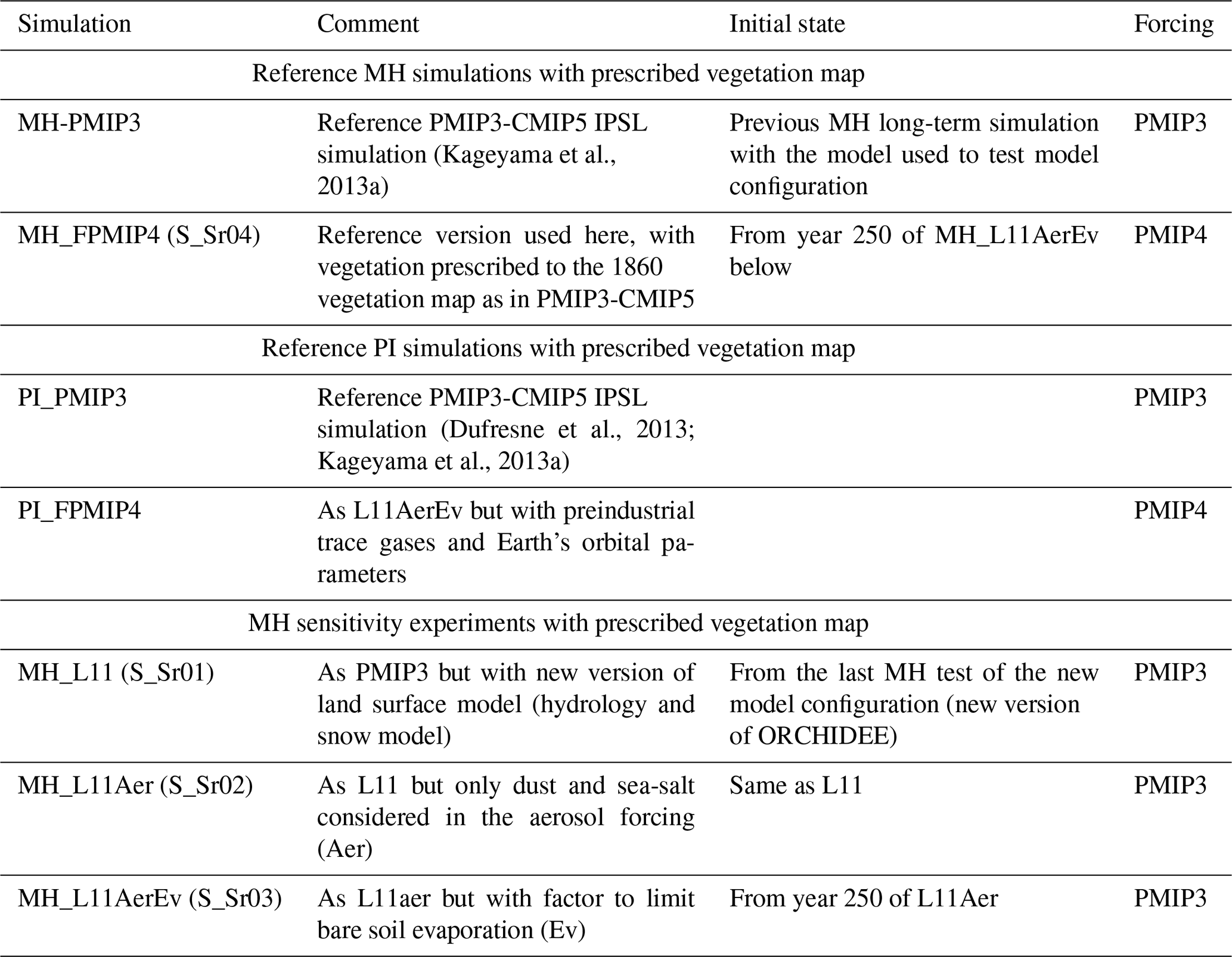
Table 2Simulations run to initialize the dynamical vegetation starting from bare soil or from vegetation map and soil moisture resulting from an off-line ORCHIDEE simulation with dynamical vegetation switched on and using the PI L11 simulated climate as boundary conditions. We include in parentheses the tag of the simulation that corresponds to our internal nomenclature for memory.
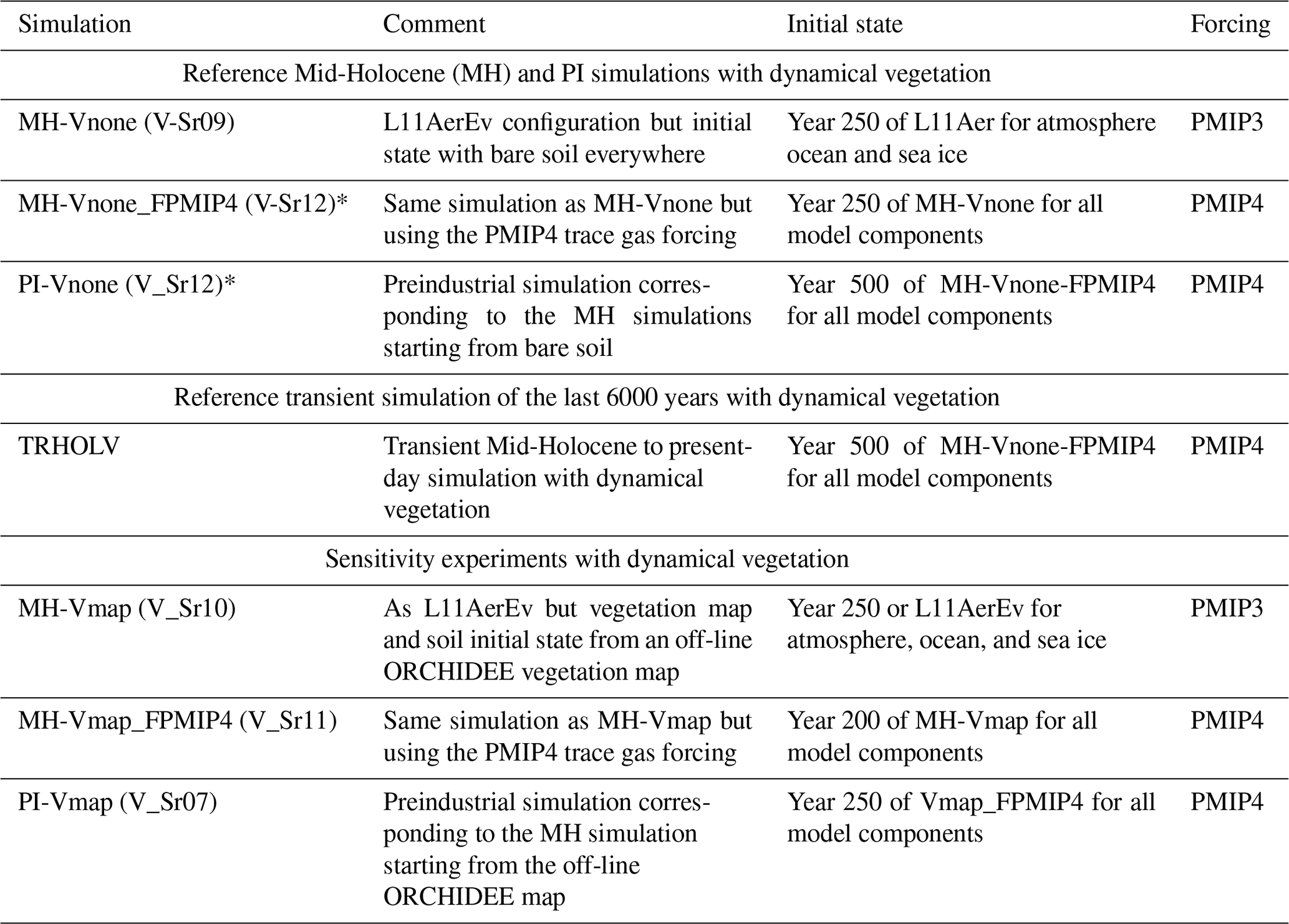
* Simulations with an asterisk are considered as references for the model version and the transient simulations.
Most tests follow the MH-PMIP3 protocol (Braconnot et al., 2012). This is only due to the fact that this work began before the PMIP4 boundary conditions were available. But the transient simulation (TRHOLV, for TRansient HOLocene simulation with dynamical Vegetation) and the 1000-year-long MH simulations with or without dynamical vegetation that were run to prepare the initial state for it follow the PMIP4-CMIP6 protocol (Otto-Bliesner et al., 2017, Table 1). In all simulations the Earth's orbital parameters are derived from Berger (1978). The MH-PMIP3 protocol uses the trace gases (CO2, CH4 and N2O) reconstruction from ice core data by Joos and Spahni (2008). It has been updated for PMIP4, using new data and a revised chronology that provides a consistent history of the evolution of these gases across the Holocene (Otto-Bliesner et al., 2017). The difference in forcing between PMIP4 and PMIP3 was estimated to be −0.8 W m−2 by Otto-Bliesner et al. (2017). This is the order of magnitude found for the imbalance in net surface heat flux at the beginning of the MH-FPMIP4 simulation. This simulation started from L11Aer run with the PMIP3 protocol (Fig. 1a). It uses the same model version but follows the PMIP4 protocol. For the subset of PI experiments Earth's orbit and trace gases are prescribed at their 1860 CE values, i.e., the beginning of the industrial era. For the MH and PI time slice experiments, boundary conditions do not vary with time. For the transient simulations the Earth's orbital parameters and trace gases are updated every year.
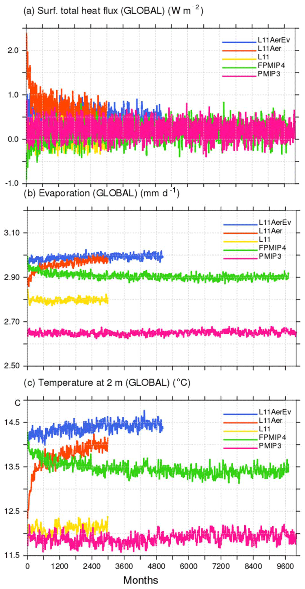
Figure 1Illustration of the effect of the different adjustments made to produce Mid-Holocene simulations with the modified version of the IPSLCM5A-MR model in which the land surface model ORCHIDEE includes a different soil hydrology and snow models (see text for details). The three panels show the global average of (a) net surface heat flux (W m−2), (b) evaporation (kg m−2), and (c) 2 m air temperature (∘C). The different colored lines represent the results for the different simulations reported in Table 1.
In standard versions of the IPSL model, aerosols are accounted for by prescribing the optical distribution of dust, sea salt, sulfate, and particulate organic matter (POM), so as to take into account the coupling between aerosols and radiation (Dufresne et al., 2013). For MH simulations these variables are prescribed at 1860 CE values, for which the level or sulfate and POM is slightly higher than the values found in the Holocene (Kageyama et al., 2013a). Here, except for the first few tests (Table 1), we prescribe only dust and sea salt at their 1860 values and neglect the other aerosols. A fully coupled dust–sea-salt–climate version of the model that does not consider the other aerosols is under development for long transient simulations. For future comparisons it is important to have a similar model setup. Indeed, compared to the version with all aerosols, considering only dust and sea salts imposes a radiative difference of about 2.5 W m−2 in external climate forcing. Its footprint appears on the net heat flux imbalance at the beginning of L11Aer. It leads to a global air temperature increase of 1.5 ∘C (Fig. 1c). The largest warming over land is found in the Northern Hemisphere, but the ocean warms almost everywhere by about 1 ∘C, except in the Antarctic circumpolar current (Fig. 2b). The warmer conditions favor higher precipitation with a global pattern rather similar to what is found in future climate projections (Fig. 2a). This offset affects the mean climate state and is larger than the expected effect of Holocene dusts.
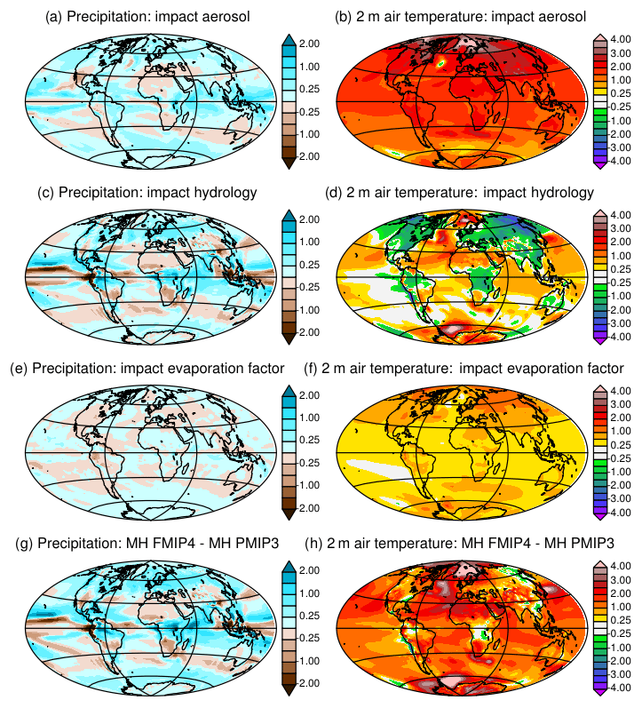
Figure 2Mid-Holocene annual mean precipitation (mm d−1) and 2 m air temperature (∘C) difference between (a, b) L11Aer and L11, (c, d) L11 and PMIP3, (e, f) PMIP3L11AerEv and L11Aer, and (g, h) FPMIP4 and PMIP3. See Table 1 and text for details on the different simulations.
2.2 The IPSL Earth system model and updated version of the land surface scheme
For these simulations, we use a modified version of the IPSLCM5A model (Dufresne et al., 2013). This model version couples the LMDZ atmospheric model with 144×142 grid points in latitude and longitude (2.5∘ × 1.27∘) and 39 vertical levels (Hourdin et al., 2013) to the ORCA2 ocean model at 2∘ resolution (Madec, 2008). The ocean grid is such that resolution is enhanced around the Equator and in the Arctic due to the grid stretching and pole shifting. The LIM2 sea-ice model is embedded in the ocean model to represent sea-ice dynamics and thermodynamics (Fichefet and Maqueda, 1999). The ocean biogeochemical model PISCES is also coupled to the ocean physics and dynamics to represent the marine biochemistry and the carbon cycle (Aumont and Bopp, 2006). The atmosphere–surface turbulent fluxes are computed taking into account fractional land–sea area in each atmospheric model grid box. The sea fraction in each atmospheric grid box is imposed by the projection of the land–sea mask of the ocean model on the atmospheric grid, allowing for a perfect conservation of energy (Marti et al., 2010). Ocean, sea ice, and atmosphere are coupled once a day through the OASIS coupler (Valcke, 2006). All the simulations keep exactly the same set of adjusted parameters as in Dufresne et al. (2013) for the ocean–atmosphere system.
The land surface scheme is the ORCHIDEE model (Krinner et al., 2005). It is coupled to the atmosphere at each atmospheric model 30 min physical time steps and includes a river runoff scheme to route runoff to the river mouths or to coastal areas (d'Orgeval et al., 2008). Over the ice sheet, water is also routed to the ocean and distributed over wide areas so as to mimic iceberg melting and to close the water budget (Marti et al., 2010). This model accounts for a mosaic vegetation representation in each grid box, considering 13 (including two crops) plant functional types (PFTs) and interactive carbon cycle (Krinner et al., 2005).
We made several changes in the land surface model (Table 1). The first one concerns the inclusion of the 11-layer physically based hydrological scheme (de Rosnay et al., 2002) that replaces the 2-layer bucket-type hydrology (Ducoudré et al., 1993). The 11-layer hydrological model had never been tested in the fully coupled mode before this study. We paid particular attention to closing the water budget of the land surface model to ensure that O (1000 years) simulations will not exhibit spurious drift in sea level and salinity. In addition, the new prognostic snow model was included (Wang et al., 2013). The scheme describes snow with three layers that are distributed so that the diurnal cycle and the interaction between snowmelt and runoff are properly represented. In order to avoid snow accumulation on a few grid points, snow depth is not allowed to exceed 3 m. The excess snow is melted and added to soil moisture and runoff while conserving water and energy (Sylvie Charbit and Christophe Dumas, personal communication, 2017). Because of a large cold bias at high latitudes in the first tests, we reduced the bare soil albedo that is used to combine fresh snow and vegetation in the snow-aging parameterization. Other changes concern the adjustments of some of the parameterizations. The way the mosaic vegetation is constructed in ORCHIDEE favors bare soil too much when leaf area index (LAI) is low (Guimberteau et al., 2018). To overcome this problem, an artificial factor of 0.70 was implemented in front of bare soil evaporation to reduce it (Table 1). This factor is compatible with the order of magnitude of the reduction brought by the implementation of a new evaporation parametrization for bare soil in the current IPSLCM6A version of the model (Philippe Peylin, personal communication, 2017). For all the other surface types the evaporation is computed as in L11. The last adjustment concerns the combination of snow albedo with the vegetation albedo. The procedure was different when vegetation was interactive or prescribed. Now the combination of snow and vegetation albedo is based on the effective vegetation cover in the grid box in both cases. It leads to a larger albedo than with the IPSL-CM5A-LR reference version when vegetation is prescribed. It counteracts the effect of the fresh snow albedo reduction.
2.3 Impact of the different changes on model climatology and performances
Figures 1 and 2 highlight how the changes discussed in Sect. 2.2 affect the model adjustment and climatology. The hydrological model (L11) produces about 1.25 mm d−1 higher global annual mean evaporative rates than MH-PMIP3. The water cycle is more active in L11. Precipitation is enhanced in the midlatitudes and over the tropical lands (Fig. 2c) where larger evapotranspiration and cloud cover both contribute to cooling the land surface (Fig. 2d). A higher evaporative rate should lead to a colder global mean temperature (Fig. 1c). This is not the case. The large-scale cooling over land is compensated for by warming over the ocean (Fig. 2d), caused by reduced ocean evaporation and changes in the ocean–land heat transport. The radiative equilibrium is achieved at the top of the atmosphere with the same global mean long-wave and shortwave radiation budget in the two simulations (L11 and MH_PMIP3).
The factor introduced to reduce bare soil evaporation did not lead to the expected reduction in evaporation (Fig. 1b). Indeed, when evaporation is reduced, soil temperature increases and the regional climate becomes warmer, allowing for more moisture in the atmosphere and thereby more evaporation where soil can supply water (Figs. 2e, f and 1). Therefore, differences resulting from bare soil evaporation do not show up on the precipitation map (Fig. 2e) but in the increased temperature over land in the Northern Hemisphere (Fig. 1f). This is consistent with similar findings when analyzing land use feedback (Boisier et al., 2012). Note that in Fig. 2f about 0.1 ∘C of the 0.4 ∘C global warming in L11AerEv is still a footprint of the warming induced by the aerosol effect described in Sect. 2.1 but that it does not alter our conclusions on the regional temperature–evaporation feedback.
The difference between MH-FPMIP4 and MH-PMIP3 represents the sum of all the changes in the land surface model and forcing discussed above (Fig. 2g, h). A PI simulation performed with the new model version (PI-FPMIP4, Table 1) allows us to assess how they affect the model performances. A rapid overview of model performances is provided by a simple set of metrics derived from the PCMDI Metric Package (Gleckler et al., 2016, see Appendix 1). Figure 3 highlights that temperature biases are reduced in PI-FPMIP4 at almost all model levels but that biases are enhanced for precipitation and total precipitable water compared to PI-PMIP3 (comparison of blue and black lines in Fig. 3). Taken together all the changes we made have little effect on the bias pattern (Fig. 3a). The model performs quite well compared to the CMIP5 ensemble of PI simulations, except for cloud radiative effect (Fig. 3). The effect of cloud in the IPSLCM5A-LR simulations results mainly from low level clouds over the ocean (Vial et al., 2013; Braconnot and Kageyama, 2015). The atmospheric tuning is exactly the same as in the default IPSLCM5A-LR version, and the introduction of all the changes described above has almost no effect on the cloud radiative effect. Overall, the model version with the 11-layer hydrology has similar skill to the IPSLCM5A reference (Dufresne et al., 2013), and we are confident that the version is sufficiently realistic to serve as a basis on which we can include the dynamical vegetation.
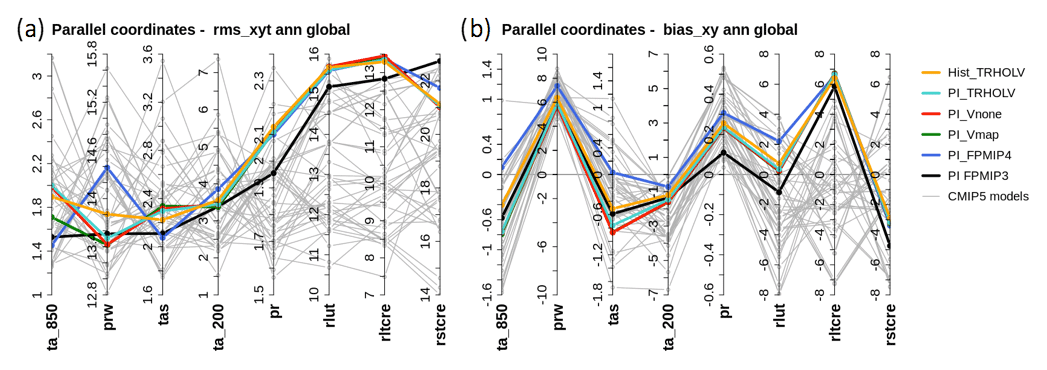
Figure 3(a) Spatiotemporal root mean square differences (rms_xyt) and (b) annual mean global model bias (bias_xy) computed on the annual cycle (12 climatological months) over the globe for the different preindustrial simulations considered in this paper (colored lines) and individual simulations of the CMIP5 multi-model ensemble (gray lines). The metrics for the different variables are presented as parallel coordinates, each of them having their own vertical axis with corresponding values. In these plots, “ta” stands for temperature (∘C) with “s” for surface (850 and 200 for 850 and 200 hPa, respectively), “prw” for total water content (g kg−1), “pr” for precipitation (mm d−1), “rlut” for outgoing long-wave radiation (W m−2), and “rltcre” and “rltcre” for the cloud radiative effect at the top of the atmosphere in the shortwave and long-wave radiation, respectively (W m−2). See Appendix A for details on the metrics.
2.4 Initialization of the Mid-Holocene dynamical vegetation for the transient simulation
We added the vegetation dynamics by switching on the dynamical vegetation model described in Zhu et al. (2015). Compared to the original scheme (Krinner et al., 2005), it produces more realistic vegetation distribution in mid- and high-latitude regions when compared with present-day observations.
Two different strategies have been tested to initialize the dynamical vegetation (Table 2). In the first case (MH-Vmap), the initial vegetation distribution was obtained from an off-line simulation with the land surface model forced by the CRU-NCEP 1901–1910 climatology. In the second case (MH-Vnone), the model restarted from bare soil with the dynamical vegetation switched on, using the same initial state as MH-Vmap for the atmosphere, the ocean, the sea ice, and the land ice. As expected, the evolution of bare soil, grass, and trees is very different in MH-Vmap and MH-Vnone during the first adjustment phase (black and blue curves in Fig. 4a–c). Vegetation adjusts in less than 100 years (1200 months) in MH-Vmap (blue curve). This short-term adjustment indicates that the climate–vegetation feedback has a limited impact on vegetation when the initial state is already consistent with the characteristics of the simulated climate. In MH-Vnone, which starts from bare soil (black curve), the adjustment has a first rapid phase of 50 years for bare soil and about 100 years for grass and trees, followed by a longer phase of about 200 years. The latter corresponds to a long-term oscillation that has been induced by the initial coupling shock between climate and land surface. Note that PMIP4 instead of PMIP3 MH boundary conditions were used to run the last part of these simulations (red and yellow curves in Fig. 4a–c). In the coupled system, most of the vegetation adjustment takes about 300 years, which is longer than results of off-line ORCHIDEE simulations (less than 200 years). Since MH-Vnone started from a coupled ocean–atmosphere–ice state at equilibrium, this result also indicates that the land–sea–atmosphere interactions do not alter the global energetics of the IPSL model much in this simulation where atmospheric CO2 is prescribed. The two simulations converge to very similar global vegetation cover. Figure 4 suggests that there is only one global mean stable state for the Mid-Holocene with the IPSL model, irrespective of the initial vegetation distribution (see also Table A1, Appendix A1).
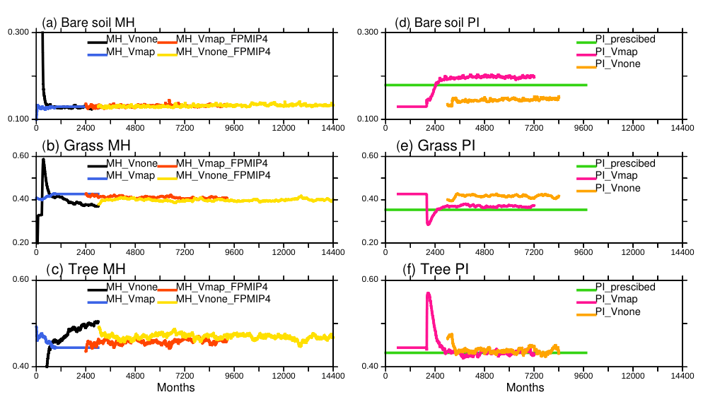
Figure 4Long-term adjustment of vegetation for the Mid-Holocene (MH)(a, b, c) and preindustrial (PI) climate(c, d, e), when starting from bare soil (Vnone) or from a vegetation map (Vmap). The 13 ORCHIDEE PFTs have been gathered as bare soil, grass, trees, and land use. When the dynamical vegetation is active, only natural vegetation is considered. Land use is thus only present in one simulation, corresponding to a preindustrial map used as a reference in the IPSL model (Dufresne et al., 2013). The corresponding vegetation is referred to as PI_prescribed. The x axis is in months, starting from 0, which allows us to plot all the simulations that have their own internal calendar on the same axis.
For the transient simulation, we decided to use the results of the MH-VNone simulation as initial state (Table 2) because it leads to more realistic forest in the PI-Vnone simulation (see discussion in Sect. 4). We performed a preindustrial simulation (PI-Vnone) using MH-Vnone as an initial state and switching on the orbital parameters and trace gases to their PI values. Figure 3 indicates that the vegetation feedback slightly degrades the global performances for PI temperature and brings the model performance close to the IPSLCM5A-LR CMIP5 version. It also contributes to reducing the mean bias in precipitable water, evaporation, precipitation, and long-wave radiation, but it has no effect on the bias pattern (assessed by the rmst (spatiotemporal root mean square error) in Fig. 3; see also Appendix). Vegetation thus has an impact on climate, but its effect is of smaller magnitude than those of the different model and forcing adjustments done to set up the model version we use here. Section 4 provides a more in-depth discussion of the vegetation state.
3.1 Long-term forcing
Starting from the MH-Vnone simulation, the transient simulation of the last 6000 years (TRHOLV) allows us to test the response of climate and vegetation to atmospheric trace gases and Earth's orbit (see Sect. 2.1). The atmospheric CO2 concentration slowly rises throughout the Holocene from 264 ppm 6000 years ago to 280 for the preindustrial climate at around −100 BP (1850 CE) and then experiences a rapid increase from −100 BP to 0 BP (1950 CE) (Fig. 5). The methane curve shows a slight decrease and then follows the same evolution as CO2, whereas NO2 remains around 290 ppb throughout the period. The radiative forcing of these trace gases is small over most of the Holocene (Joos and Spahni, 2008). The largest changes occurred with the industrial revolution. The rapid increase in the last 100 years of the simulation has an imprint of about 1.28 W m−2.

Figure 5Evolution of trace gases CO2 (ppm), CH4 (ppb), and N2O (ppb) and seasonal amplitude (maximum annual – minimum annual monthly values) of the incoming solar radiation at the top of the atmosphere (W m−2) averaged over the Northern Hemisphere (black line) and the Southern Hemisphere (red line). These forcing factors correspond to the PMIP4 experimental design discussed by Otto-Bliesner et al. (2017).
The major forcing is caused by the slow variations in the Earth's orbital parameters that induce a long-term evolution of the magnitude of the incoming solar radiation seasonal cycle at the top of the atmosphere (Fig. 5). It corresponds to decreasing seasonality (difference between the maximum and minimum monthly values for each year) in the Northern Hemisphere and increasing seasonality in the Southern Hemisphere (Fig. 5). It results from the combination of the changes in summer and winter insolation in both hemispheres (Fig. 6). These seasonal changes are larger at the beginning of the Holocene (about −8 W m−2 per millennium in the Northern Hemisphere, NH, and +5 W m−2 per millennium in the Southern Hemisphere, SH) and then the rate of change linearly decreases in the NH (increases in the SH) from 4500 to about 1000 BP (Fig. 5). There is almost no change in seasonality in the NH over the last 1000 years, whereas in the SH seasonality starts to decrease again by 2000 BP. The shape of insolation changes is thus different in both hemispheres and so is the relative magnitude of the seasonal cycle between the two hemispheres. This would be seen whatever the calendar we used to compute the monthly means because of the seasonal asymmetry induced by precession in the MH (see Joussaume and Braconnot, 1997; Otto-Bliesner et al., 2017).
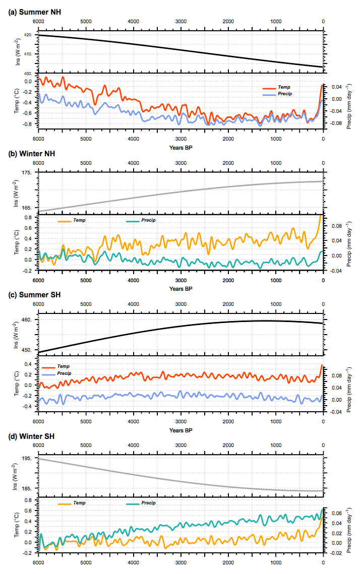
Figure 6Long-term evolution of incoming solar radiation at the top of the atmosphere (TOA) (W m−2; upper section of panels) and associated response of temperature (∘C) and precipitation (mm yr−1) expressed as the difference to the 6000 BP initial state and smoothed by a 100-year running mean) for (a) NH summer, (b) NH winter, (c) SH summer, and (d) SH winter. Temperatures are plotted in red and precipitation in blue for summer, and they are, respectively, plotted in orange and green for winter. NH summer and SH winter correspond to June to September averages, whereas NH winter and SH summer correspond to December to March averages. All curves, except insolation, have been smoothed by a 100-year running mean.
3.2 Long-term climatic trends
Changes in temperature and precipitation follow the long-term insolation changes in each hemisphere during summer until about 2000 to 1500 BP (Fig. 6). Then trace gases and insolation forcing become equivalent in magnitude and small compared to MH insolation forcing, until the last period where trace gases lead to a rapid warming. The NH summer cooling reaches about 0.8 ∘C and is achieved in 4000 years. The last 100-year warming reaches 0.6 ∘C and almost counteracts, for this hemisphere and season, the insolation cooling. SH summer (JJAS) and NH winter (NDJF) temperatures are both characterized by a first 2000-year warming. It reaches about 0.4 ∘C. It is followed by a plateau of about 3000 years before the last rapid increase of about 0.6 ∘C that reinforces the effect of the Holocene insolation forcing. During SH winter, temperature does not seem to be driven by the insolation forcing (Fig. 6d). In both hemispheres. summer precipitation trends correlate well with temperature trends, as is expected from a hemispheric first-order response driven by a Clausius–Clapeyron relationship (Held and Soden, 2006). This is not the case for winter conditions because one needs to take into account the changes in the large-scale circulation that redistribute heat and energy between regions and hemispheres (Braconnot et al., 1997; Saint-Lu et al., 2016).
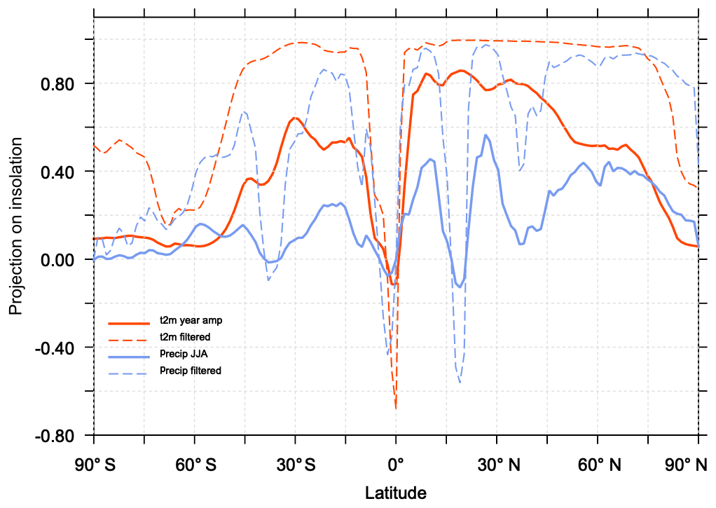
Figure 7Fraction of the evolution of the seasonal amplitude of temperature (red) and precipitation (blue) represented by the projection of these climate variables on the evolution of the seasonal amplitude of insolation as a function of latitude. The solid line stands for the raw signal and the dotted line for the signal after a 100-year smoothing.
We further estimate the links between the long-term climate response and the insolation forcing for the different latitudinal bands by projecting the zonal mean temperature and precipitation seasonal evolution on the seasonal evolution of insolation. We define the seasonal amplitude for each year as the difference between the maximum and minimum monthly values. We consider for each latitude the unit vector S:
where represents the norm of the seasonal magnitude of the incoming solar radiation at TOA over all time steps (SWis−TOA(t); years to 0, with an annual time step). Any climatic variable (V) can then be expressed as
with
where b is the unit vector orthogonal to S. The ratio measures in which proportion a signal projects onto the insolation (Fig. 7). Figure 7 confirms that the projection of temperature and precipitation onto the insolation curve is larger in the Northern than in the Southern Hemisphere. The best match is obtained between 10 and 40∘ N where about 80 % of the temperature signal is a direct response to the insolation forcing. The projections are only 50 % in the tropics in the Southern Hemisphere. These numbers go up to 90 % if a 100-year smoothing is applied to temperature. Seasonal precipitation is also projected to be as high as 90 % when considering the filtered signal, confirming the strong links between temperature and precipitation in the NH over the long timescale. The projection is poorer, but not zero, when the raw precipitation signal is considered. At the Equator and at high latitudes in both hemispheres the projection is poor or zero. At the Equator, the MH insolation forcing favors a larger north–south seasonal march of the ITCZ (Intertropical Convergence Zone) over the ocean and the inland penetration of Afro-Asian monsoon precipitation during boreal summer. Surface temperature is reduced in regions where precipitation is enhanced due to the combination of increased cloud cover and increased surface evaporation (Joussaume et al., 1999; Braconnot et al., 2007a). When the monsoon retreats to its modern position, surface temperature in these regions increases, thereby enhancing the monsoon's seasonal cycle. It is thus out of phase compared to insolation forcing. This is also true over SH continents where temperatures in regions affected by monsoons do not follow the local insolation and have a similar seasonal evolution to the Northern Hemisphere. This out-of-phase relationship is consistent with glacier reconstructions (Jomelli et al., 2011). At a higher latitude the projection of the raw signal is not good because of the large decadal variability. North of 40∘ N the mixed layer depth is also larger (about 200 m) than in the tropics (about 70 m), which contribute to damping the seasonal change over the ocean. Thus the seasonal temperature response is flatter than the shape of the seasonal insolation forcing, which leads to a poor projection over midlatitude and high-latitude ocean especially in the ocean-dominated SH (Fig. 7). Sea-ice cover has also little change north of 80∘ N, which also damps the changes in seasonality (Fig. 8). These changes are, however, amplified by the increase in sea ice during summer in the Arctic resulting from cooler conditions with time and by the reduction in the winter sea-ice cover in the Labrador and the Greenland–Iceland–Nordic seas (Fig. 8a, b). For snow cover the conditions are contrasted depending on the regions (Fig. 8a, b, d), with an decrease in the maximum cover over Eurasia related to a long-term rise in minimum temperature (Fig. 8d)
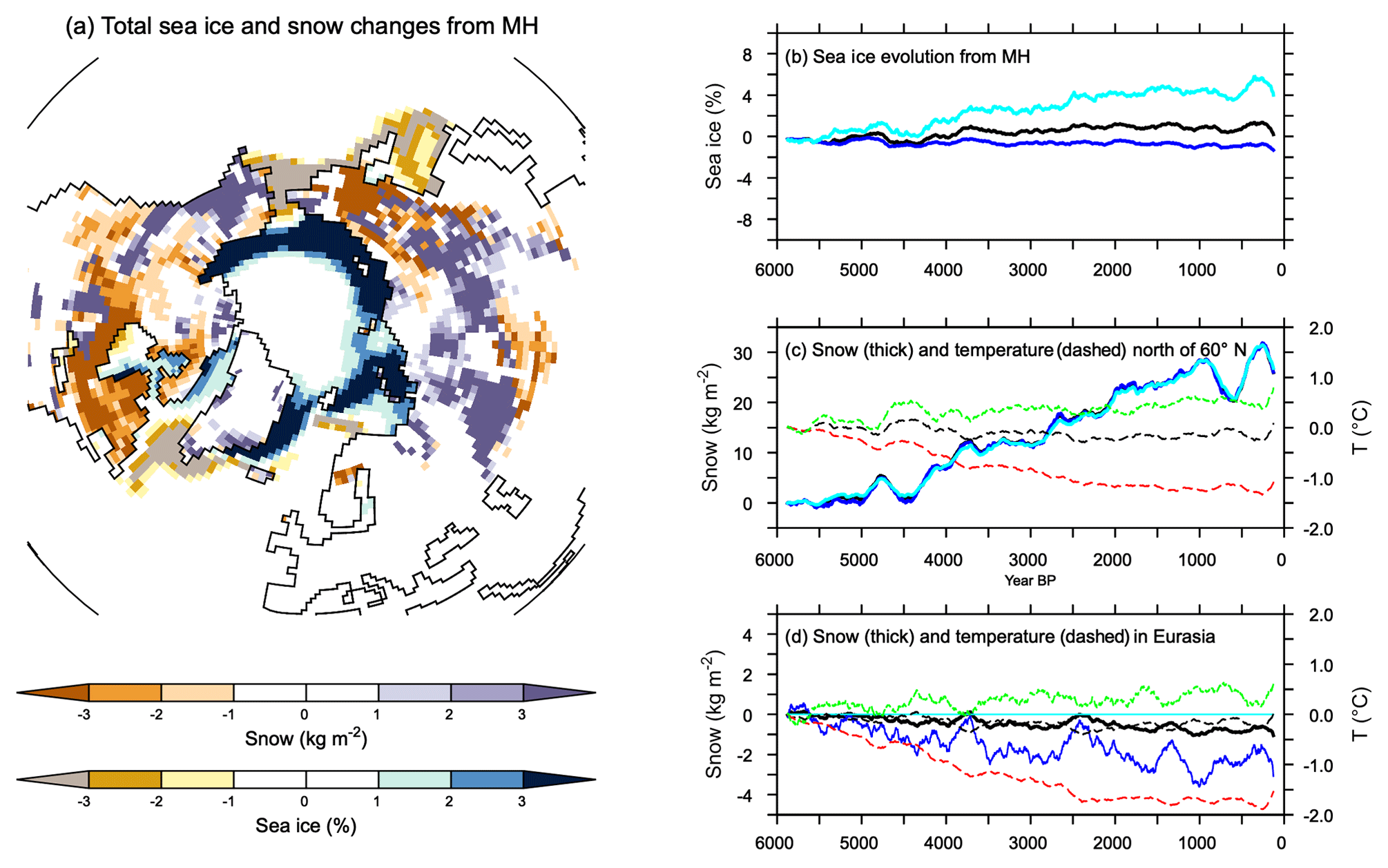
Figure 8(a) Total change in snow cover (kg m−2) and sea-ice fraction (%) integrated over the last 6000 years, and evolution from the Mid-Holocene of annual mean maximum summer and minimum winter values for (b) sea-ice averages over the Northern Hemisphere, (c) snow (solid lines) and 2 m air temperature (dotted lines) averaged for all regions north of 60∘ N, and (d) snow and 2 m air temperature over Eurasia. In (b, c), and (d) black, dark blue and light blue stand, respectively, for the annual mean, maximum, and minimum annual monthly values for sea-ice or snow cover, and black, green, and red stand for annual mean, minimum, and maximum air temperature.
3.3 Long-term vegetation trends
These long-term climate evolutions have a counterpart on the long-term evolution of vegetation (Fig. 9). At the global and hemispheric scale, the long-term vegetation trends correspond to reductions or increases in the area covered by vegetation, reaching 2 % to 4 % of the total land area depending on vegetation type (Fig. 9). The global vegetation averages reflect the Northern Hemisphere changes where most of the vegetated continental masses are located. As expected from the different long-term trends in insolation, the long-term evolution of tree and grass cover is the opposite in the two hemispheres. Note, however, that bare soil slightly increases in both hemispheres.
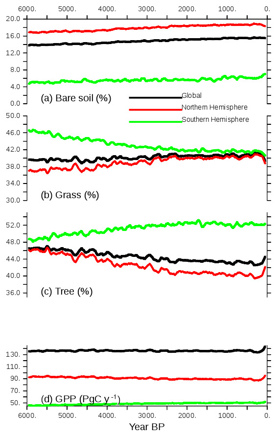
Figure 9Long-term evolution of the simulated (a) bare soil, (b) grass, and (c) tree covers, expressed as the percentage (%) of global, NH, or SH continental areas, and (d) GPP (PgC yr−1) over the same regions. Annual mean values are smoothed by a 100-year running mean.
In the Northern Hemisphere the changes follow the changes in summer temperature, with the best match obtained for grass, which increases almost linearly until 2000 BP and then remains quite stable. In the Southern Hemisphere the phasing between vegetation change and temperature is not as good, again because this hemisphere is dominated by ocean conditions rather than land conditions. However, the tree expansion reaches a maximum between 2000 and 1000 BP, and then the tree cover slightly decreases, which corresponds to the slight cooling in SH summer temperature. The gross primary productivity (GPP; Fig. 9d) is driven in both hemispheres by the changes in tree cover. It accounts for a reduction of about 5 PgC yr−1. It is, however, possible that the GPP change is misestimated in this simulation because CO2 is prescribed in the atmosphere, which implies that the carbon cycle is not fully interactive. Figure 10 compares the vegetation map obtained for the preindustrial period in TRHOLV (150–100 BP) with MH vegetation. It shows that bare soil increases in semiarid regions in Africa and Asia as well as in southern Africa and Australia. The reduction in tree PFTs is maximal north of 60∘ N, in south and southeast Asia, the Sahel, and most of North America. Tree PFTs are replaced by grass PFTs. In the Southern Hemisphere, forest cover increases in southern Africa, southeast South America, and part of Australia.
In the last 100 years the effect of trace gases and in particular the rapid increase in the atmospheric CO2 concentration leads to a rapid vegetation change characterized by tree regrowth, which is dominant in the NH (Figs. 9 and 10). This tree recovery counteracts the reduction from the Mid-Holocene in mid- and high NH latitudes (Fig. 10b, e, and h). This effect is consistent with the observed historical growth in gross primary production discussed by Campbell et al. (2017). The GPP increase in the last 100 years results from increased atmospheric CO2. It suggests that the CO2 effect counteracts the tree decline induced by insolation. When reaching 0 BP (1950 CE), bare soil remains close to PI, grass is reduced by 3 %, and trees are increased by about 3 %.
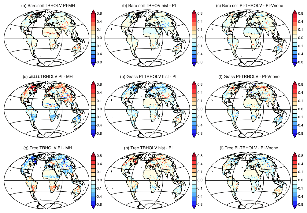
Figure 10Vegetation map comparing (a, d, g) the Mid-Holocene (first 50 years) and the preindustrial (50 years around 1850 CE (150 to 100 BP)) periods of the transient simulation, (b, d, h) the differences between the historical period (last 50 years) and the preindustrial period of the transient simulation, and (c, f, i) the difference between preindustrial climate for the transient simulation and the PI-Vnone simulations. For simplicity we only consider bare soil (a–c), grass (d–f), and trees (g–i).
3.4 Regional trends
Figure 11 highlights the long-term vegetation trends for three regions that, respectively, represent climate conditions north of 60∘ N, over the Eurasian continent, and in the West African monsoon Sahel–Sahara region. These are regions for which there are large differences in MH–PI climate and vegetation cover (Figs. 9 and 10). They have also been chosen because they are widely discussed in the literature and are also considered as tipping points for future climate change (Lenton et al., 2008). They are well suited to provide an idea of different characteristics between regions.
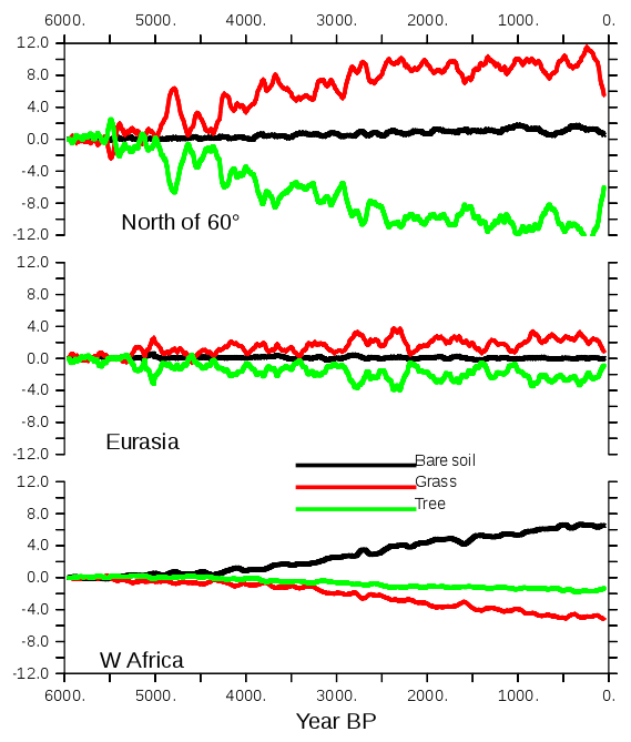
Figure 11Long-term evolution of bare soil, grass, and trees, expressed as the percentage of land cover north of 60∘ N, over Eurasia, and over West Africa. The different values are plotted as differences with the first 100-year averages. A 100-year running mean is applied to the curves before plotting.
North of 60∘ N a substantial reduction in trees at the expense of grass starts at 5000 BP (Fig. 11a, b). Vegetation almost reaches its preindustrial conditions around 2500 BP. The largest trends are found between 5000 and 2500 BP in this region, and this reflects the timing of the NH summer cooling well. The change in total forest in Eurasia is small. A first change is followed by a second one around 3000 BP. Despite the 100-year smoothing applied to all the curves, they exhibit large decadal to multi-centennial variability. Over West Africa (Fig. 11c), the largest trends start slightly later (4500–5000 BP) and are more gradual until 500 BP. The vegetation trends are also punctuated by several centennial events that do not alter the long-term evolution as much as some of these events do in the other two boxes.
The variability found for vegetation is also found in temperature and precipitation at the hemispheric scale (Fig. 6). It is even higher at the regional scale in midlatitudes and high latitudes (Fig. 8). This variability is not present in the imposed forcing. It results from internal noise. Because of this it is difficult, for example, to say whether the NH winter temperature trend was rapid until 4000 BP and then temperature remains stable or whether the event impacting temperature and precipitation around 4800 to 4500 BP masks a more gradual increase until 3000 BP, as is the case for NH summer where the magnitude of the temperature trend is larger than its variability (Fig. 6). Note that some of these internal fluctuations reach half of the total amplitude of the regional vegetation trends (Fig. 11) and that they are a dominant signal over Eurasia, where the long-term mean change in the total tree cover is small (Figs. 10 and 11). Temperature and precipitation are well correlated at this centennial timescale (Fig. 6).
Despite the dry bias over the Sahel region in this version of the model, the timing of the vegetation changes over West Africa reported in Fig. 11 is consistent with the major features discussed for the end of the African humid period (Liu et al., 2007; Hély et al., 2014). In particular, the replacement of grass by bare soil starts earlier than the reduction in the tree cover located further south (Fig. 11). At the scale of the Sahel region, we do not have abrupt changes in vegetation but gradual ones. It is, however, abrupt at the grid cell level. These changes are associated with the long-term decline in precipitation, as well as the southward shift of the tropical rain belt associated with the African monsoon (Fig. 12). The location (latitude) of the rain belt is estimated here as the location of the maximum summer precipitation zonally averaged between 10∘ W and 20∘ E over West Africa. Most of the southward shift of the rain belt occurs between MH and 3500 BP and corresponds to a difference of about 1.8∘ N of latitude over this period. Then the southward shift is smaller, with a total shift of 2.5∘ N of latitude diagnosed in this simulation. The comparison of Figs. 11 and 12 clearly shows that the rapid decrease in vegetation occurs after the rapid southward shift of the rain belt. An interesting point is that the amount of precipitation is also shifted in time compared to the location of the rain belt. It suggests that the vegetation feedback on precipitation is still effective during the first period of precipitation decline and that it might have amplified the reduction in precipitation when vegetation is reduced over the Sahel region.
As seen in Fig. 10, the NH decrease in forest cover is mainly driven by the changes that occur north of 60∘ N (Figs. 8 and 10). These trends reflect more or less what is expected from observations (Bigelow et al., 2003; Jansen et al., 2007; Wanner et al., 2008). It results from the summer cooling that affects both the summer sea-ice cover in the Arctic, the summer snow cover over the adjacent continent, and the amplification of the insolation forcing south of 70∘ N by snow–vegetation albedo feedback. Further south over Eurasia, Fig. 11 suggests that there are only marginal changes in Eurasia in terms of vegetation. Figure 13 shows that the total tree cover over this region does not reflect the mosaic vegetation and forest composition well. Indeed, the long-term decrease in forest is dominated by the decrease in temperate and boreal deciduous trees. Boreal needleleaf evergreen trees do not change, whereas the temperate ones increase. This figure also highlights that the long-term change in Eurasian tree composition throughout the Mid- to late Holocene is punctuated by centennial variability. The different trees also have different timing and variability. Boreal forests are more sensitive to variability during the first 3000 years of the simulation, whereas temperate broadleaf trees exhibit larger variability in the second half. The large events have a climatic counterpart (Fig. 8), so that the composition of the vegetation is a result of a combined response to the long-term climatic change and to variability. These two effects can lead to different vegetation composition depending on stable or unstable vegetation states (Scheffer et al., 2012). Decadal vegetation changes have been discussed for recent climate in these regions (Abis and Brovkin, 2017), which suggests that despite the fact that our dynamical vegetation model might underestimate vegetation resilience, the rapid changes in vegetation mosaic are a key signal over Eurasia. Future model–data comparisons should consider composition changes and variability to properly discuss vegetation changes over this region.
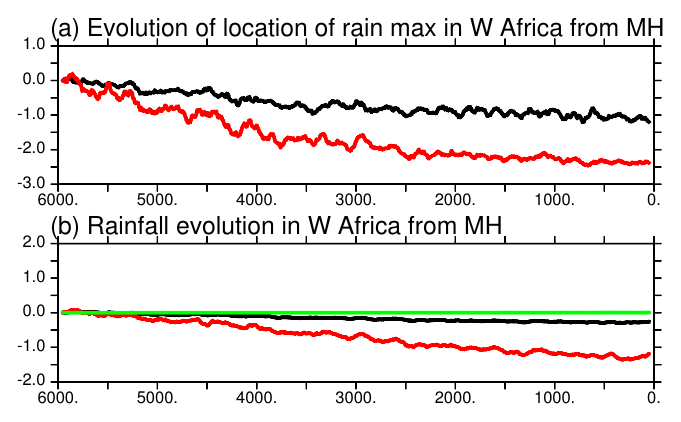
Figure 12Evolution of (a) the location of the West African monsoon annual mean (black) and maximum (red) rain belt in degrees of latitude and (b) annual mean (black), minimum (green), and maximum (red) monthly precipitation (mm d−1) averages over the Sahel region. The first 100 years have been removed and a 100-year running mean applied before plotting.
4.1 Simulated versus reconstructed vegetation
Section 3 shows how climate and vegetation respond to insolation and trace gases. The simulated changes are in broad agreement with what is expected from various sources of data. However, Sect. 2 mentions model adjustments and biases. They all contribute to the difficulty of producing the right vegetation changes in the right place, at the right time, and for the right reasons. It is thus important to fully understand what we can expect in terms of realism from this simulation. We investigate it for the Mid-Holocene and modern climate, for which we can use the BIOME6000 vegetation reconstruction (Harrison, 2017).
The dynamical vegetation module simulates fractional cover of 13 PFTs. These PFTs cannot be directly compared with the reconstructed biome types based on pollen and plant macrofossil data from the BIOME 6000 dataset (Harrison, 2017). In order to facilitate the comparison, we converted the simulated PFTs into eight mega-biomes, using the biomization method algorithm proposed by Prentice et al. (2011). The algorithm uses a mixture of simulated climate and vegetation characteristics (see Appendix and Fig. A2). Alternative thresholds as proposed in previous studies (Joos et al., 2004; Prentice et al., 2011) were tested to account for the uncertainties in the biomization method (see Fig. A2). At a first glance MH-Vnone reproduces the large-scale pattern found in the BIOME6000 reconstruction (Fig. 14a). The comparison, however, indicates that the boreal forest tree line is located too far south. It results from a combination of a cold bias in temperature in these regions and a systematic underestimation of forest biomass in Siberia with ORCHIDEE when forced by observed present-day climate (Guimberteau et al., 2018). Such underestimation of tree biomass could lead to too low a tree height in ORCHIDEE and thus to the replacement of boreal forest by dry woodland according to the biomization algorithm (Fig. A2a). Also, vegetation is underestimated in West Africa, consistent with a dry bias (not shown). The underestimation of the African monsoon precipitation is present in several simulations with the IPSL model (Braconnot and Kageyama, 2015) and is slightly enhanced in summer when the dynamical vegetation is active. With interactive vegetation, however, equatorial Africa is more humid (Fig. 15a). Figure 14c provides an idea of the major mismatches between simulated vegetation and the BIOME6000 reconstructions. In particular, the simulation produces too much desert where we should find grass and shrubs. It also produces too much tundra instead of boreal forest and too much savannah and dry woodland in several places that should be covered by temperate trees, boreal trees, or tundra, confirming the visual map comparison (Fig. 14c). Similar results are found when considering the preindustrial climate in TRHOLV compared to the BIOME6000 preindustrial biome reconstruction (Fig. A2d). These are systematic biases. These systematic biases are confirmed when comparing the simulated PFTs for PI with those of the 1860 CE map estimated from observations and used in simulations with prescribed vegetation (see Table A1 for regions without land use).
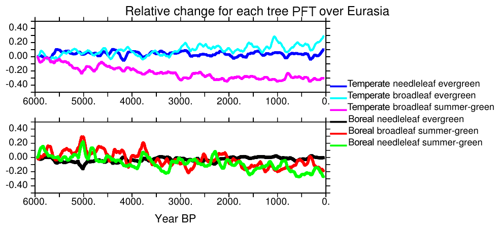
Figure 13Evolution of the different tree PFTs in Eurasia, expressed as the percentage change compared to their 6000 BP initial state. Each colored line stands for a different PFT. Values have been smoothed by a 100-year running mean.
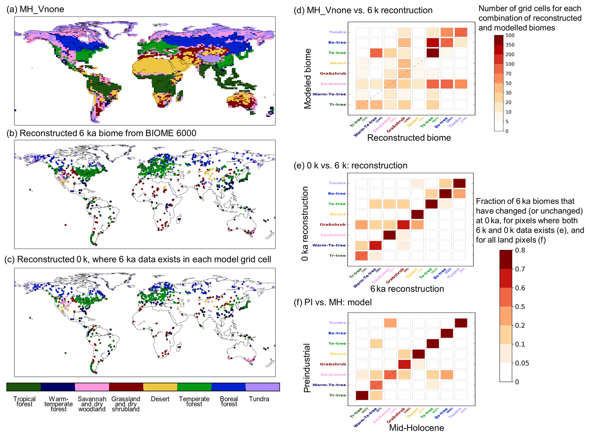
Figure 14(a) Simulated mega-biome distribution by MH-Vnone, converted from the modeled PFT properties using the default algorithm described in Fig. A1. Panels (b) and (c): reconstructions in BIOME 6000 DB version 1 for the MH and PI periods (Harrison, 2017). (d) Number of pixels where reconstruction is available and the model matches (or does not match) the data. Note that multiple reconstruction sites may be located in the same model grid cell, in which case we did not group them so that each site was counted once. Numbers in parentheses on the x axis in (d) represent the number of sites for each biome type. Panel (e) same as (c) but for the number of matches between (e) the BIOME6000 MH (6 k) and PI (0 k) reconstructions at pollen sites and (f) the simulated mega-biomes for MH and PI at each model grid cell.
It is not possible to estimate the vegetation feedback on the long-term climate evolution from the transient simulation. It is, however, possible to infer how the dynamical vegetation affects the mean climatology for the MH, a period for which simulations with prescribed and dynamic vegetation are available. Metrics discussed in Sect. 2.4 (Fig. 3) show that the introduction of the dynamical vegetation in the model reduces the amount of precipitation and that the climate is dryer. The simulations with dynamical vegetation only consider natural vegetation, whereas the 1860 CE map we prescribe when vegetation is fixed includes land use. In regions affected by land use, all MH simulations produce less bare soil (3 %), more tropical trees (5 %), similar temperate tree cover, increased boreal tree cover (10 %), and a different distribution between C3 versus C4 grass (see Table A1). In Eurasia where croplands are replaced by forest, the lower forest albedo induces warmer surface conditions (Fig. 15b). Also, when snow combines with forest instead of grasses, the snow–vegetation albedo is lower, leading to the positive snow–forest feedback widely discussed for the last glacial inception (de Noblet et al., 1996; Kutzbach et al., 1996). Figure 15a also highlights that precipitation is increased over the African tropical forest and reduced over South America. In most regions the impact of vegetation is much smaller than the impact of the changes in the land surface hydrology and forcing strategy discussed in Sect. 2.3 (Fig. 2).
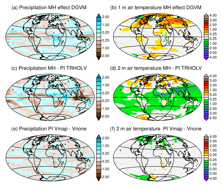
Figure 15Impact of the dynamical vegetation and initialization of vegetation on the simulated climate. Differences for annual mean (a, c, e) precipitation (mm d−1) and (b, d, f) 2 m air temperature (∘C) between (a) the MH in the TRHOLV simulation and (b) the MH simulation without dynamical vegetation (MH FPMIP4), (c) the Mid-Holocene and (d) the preindustrial simulations in the TRHOLV simulation, and (e) and (f) the two preindustrial simulations initialized from bare soil (PI-Vnone) or a vegetation map for vegetation (PI-Vmap). See Table 2 and text for details on the simulations.
The differences between the MH simulated vegetation map and the 1860 CE map reflect both systematic model biases and vegetation changes related to the MH climate differences with PI. We can infer from Figs. 15 and 16 that vegetation has a positive warming feedback in the high latitudes during MH. Part of the differences between the MH and the PI conditions in Fig. 15c, d is dominated by the impact of vegetation. Similar patterns as those obtained for the impact of vegetation are found over Eurasia for temperature, or southeast Asia and North America for precipitation. For the grid points where BIOM6000 data are available for both MH and PI (0 k – 1860 CE), the major simulated biome changes occur for savannah and wood and grass and shrubs (Fig. 14e). Differences are also found for trees and tundra, but to a lesser extent. The comparison with similar estimates from BIOME6000 reconstructions indicates that grass and shrubs exhibit major changes and that trees show larger differences compared to the simulation. The model shift between savannah and wood and grass and shrubs is consistent with the noted bias for savannah and the fact that the tree cover is underestimated in NH latitudes (Fig. 14).
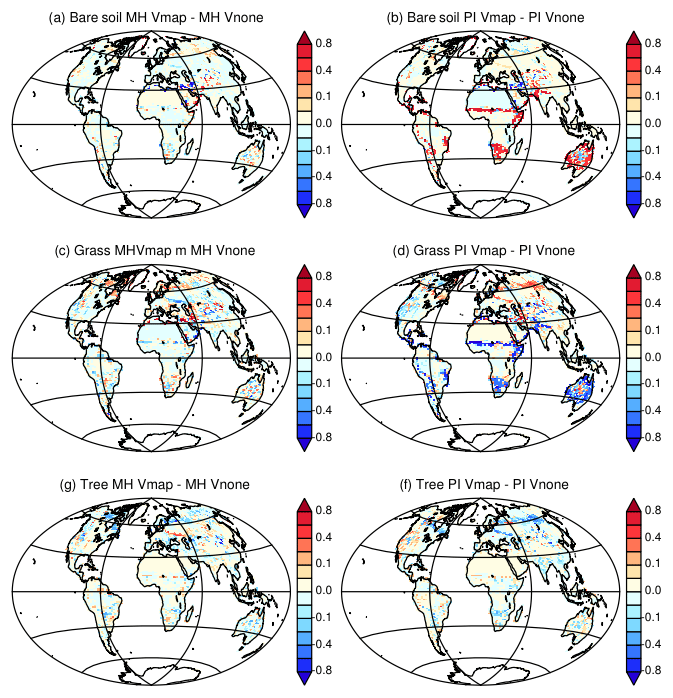
Figure 16Difference between Vegetation maps obtained with the two different initial states for (a, c, e) Mid-Holocene simulations and (b, d, f) preindustrial simulations. Vmap stands for MH and PI simulations where the Mid-Holocene vegetation has been initialized from a vegetation map and Vnone for MH and PI simulations where the Mid-Holocene has been initialized from bare soil. For simplicity we only consider fractions of (a, b) bare soil, (c, d) grass, and (e, f) trees.
Note that the vegetation differences found between the historical period and the PI period in TRHOLV are not negligible. We can estimate from Fig. 15a, b that neglecting land use leads to an underestimation of about 1 ∘C in Eurasia between the MH and PI in this TRHOLV simulation. Depending on whether PI or the historical period is used as a reference, the magnitude of the MH changes in vegetation and climate are different. Also, land use has regional impacts and should be considered in PI or in the historical period. This stresses that a quantitative model–data comparison must be treated with caution, knowing that both the reference period (PI or historical) and the complexity of the land surface model (prescribed vegetation, natural dynamical vegetation, land use … ) can easily lead to 1 ∘C difference in some regions.
4.2 Multiple vegetation states for the preindustrial climate
Another source of uncertainty concerns the stability of the simulated vegetation maps. Several studies suggest that the initial state only has a minor impact on the final climate because there is almost no change in the thermohaline circulation over this period and models do not exhibit major climate bifurcations (e.g., Bathiany et al., 2012). This is the main argument used by Singarayer and Valdes (2010) to justify that their suite of snapshot experiments may provide a reasonable transient climate vision when put together. Is this the case in the TRHOLV simulation when vegetation is fully interactive? This transient simulation does not exhibit much change in the indices of thermohaline circulation, which remains close to 16–18 Sv (sverdrup) (1 Sv =106 m3 s−1) throughout the period. The global metrics (Fig. 3) show that at the global scale the results of the TRHOLV simulations for PI (1860 CE) are similar to those of PI-Vnone. It is also the case for seasonal and extratropical or tropical values (Fig. A1). We can therefore conclude that there is no difference in mean surface climate characteristics between the snapshot PI-Vnone experiments and the PI period simulated in the transient TRHOLV simulation.
Is the vegetation then also similar to the one simulated in PI-VNone? The PI vegetation simulated in TRHOLV shows little differences to the one found for PI-Vnone (Fig. 10c, f, and i). The relative percentages of land covered by the different vegetation classes correspond to 15 % for bare soil, 41 % for grass, and 43 % for trees, respectively. These values are similar to the one found for PI-VNone (15 %, 40 %, and 44 %, respectively) within 1 % error bar. This does not necessarily hold at the regional scale where regional differences are also found between PI-TRHOLV and PI-Vnone. Indeed, Fig. 10 indicates differences in tree and grass cover in Eurasia around 60∘ N and different geographical coverage between bare soil, grass, and trees over southern Africa and Australia. These differences are very small compared to the differences between MH and PI in TRHOLV, but are as large as the difference between historical (i.e., the last 50 years of the simulation) and PI in a few places in Eurasia. As seen in previous section, these are regions where variability is large and vegetation instable.
We also tested whether the PI vegetation and climate would also be similar when starting from MH-Vmap instead of MH-Vnone (dark pink and orange lines in Fig. 4d–f). This is also a way to have a better idea of the range of response one would expect from ensemble simulations, knowing that we only ran one full transient simulation. For the PI-Vmap simulation, the orbital parameters and trace gases were first prescribed to preindustrial conditions for 15 years while maintaining the vegetation PFTs in each grid cell to those obtained in MH-Vmap (Table 2, Fig. 4). Then, the dynamical vegetation was switched on. It induces a rapid transition of the major PFTs that takes about 10 years before a new global equilibrium is reached (Fig. 4d–f). For PI-VNone presented in Sect. 2.4 the same procedure was applied, but the dynamical vegetation was switched on after 5 years (Table 2 and Fig. 4), and the new equilibrium state is reached without any relaxation or rapid transition.
PI-Vnone and PI-Vmap converge to different global vegetation states (Fig. 4). Compared to the values listed above for PI-Vnone and PI-TRHOLV the respective covers of bare soil, grass, and trees for PI-Vmap are 20 %, 37 %, and 43 %. In particular, PI-Vmap produces a larger bare soil cover than PI-Vnone (Fig. 4d). It is even larger than the total bare soil cover found in the 1860 CE map used in PI simulations when vegetation is prescribed (Fig. 4). Interestingly part of these differences between Vmap and Vnone is found in the Southern Hemisphere and the northern edge of the African and Indian monsoon regions. Since there is almost no difference in MH vegetation between Vmap and Vnone, these differences in PI vegetation drive the vegetation differences between MH and PI (Fig. 16). The MH simulated changes seem larger with Vmap. A previous assessment of model results against vegetation and paleoclimate reconstructions (e.g., Harrison et al., 1998, 2014) suggests that MH–PI vegetation for Vmap would be in better agreement with reconstructed changes from observations in terms of forest expansion in the Northern Hemisphere or grasses in the Sahel (Fig. 16). However, the modern vegetation map for this PI-Vmap simulation has even less forest than PI-Vnone north of 55∘ N (Fig. 4e, f, and i), for which forest is already underestimated (Fig. A2). These differences in PI vegetation only have a small counterpart in climate. These biases correspond to cooler condition in the midlatitudes and high northern latitude (Fig. 15). In the annual mean, there is almost no impact on precipitation (Fig. 15). In terms of climate these two simulations are very similar and closer to each other than to other simulations, whatever the season or the latitudinal band (Fig. A1). The small differences in climate listed above are thus too small to be captured by global metrics. It suggests that there is no direct relationship between the different vegetation maps and model performances. The different vegetation maps are obtained with a similar climate, which indicates that in this model multiple global and vegetation states are possible under preindustrial climate or that tiny climate differences can lead to different vegetation.
This long transient simulation over the last 6000 years with the IPSL climate model is one of the first simulations over this period with a general circulation model including a full interactive carbon cycle and dynamical vegetation. Several adjustments were made to set up the model version and the transient simulations. Most of them have a larger impact on the model climatology than the dynamical vegetation feedback and remind us that fast feedbacks occur in coupled systems so that any evaluation of surface flux should consider both the flux itself and the climate or atmospheric variables used to compute it (Torres et al., 2018). We show that, despite some model biases that are amplified by the additional degree of freedom resulting from the coupling between vegetation and climate, the model reproduces reasonably well the large-scale features in climate and vegetation changes expected from reconstructions over this period. The transient simulation exhibits little change in annual mean climate throughout the last 6000 years (not shown). The seasonal cycle is the main driver of the climate and vegetation changes, except in the last part of the simulation when the rapid greenhouse gas concentration increase leads to rapid global warming. There has been lots of discussion regarding the sign of the trends in the northern midlatitudes following the results of the first coupled ocean–atmosphere simulation with the CCSM3 model across deglaciation (Liu et al., 2014). Our results seem in broad agreement with the 6000 to 0 BP part of the revised estimates by Marsicek et al. (2018).
The analysis of vegetation differences between PI-Vmap and PI-VNone once more raises the possibility of multiple vegetation equilibrium under preindustrial or modern conditions, as has been widely discussed previously (e.g., Brovkin et al., 2002; Claussen, 2009). Here we have both global and regional differences. Our results are, however, puzzling because we only find limited differences between the PI-Vnone snapshot simulation and the PI climate and vegetation produced at the end of TRHOLV. These simulations start from the same initial state and in one case PI conditions are switched on in the forcing, whereas in the other case the 6000-year long-term forcing in insolation and trace gases is applied to the model. An ensemble of simulations would be needed to fully assess vegetation stability. In the Northern Hemisphere and over forest areas, MH-Vmap produced slightly fewer trees that MH-Vnone. It might have been amplified by snow–albedo feedback under the PI conditions that are characterized by a colder than MH climate at high latitudes in response to reduced incoming solar radiation associated with lower obliquity. The differences between the Southern Hemisphere and the Northern Hemisphere characterized by large differences in grasses and bare soil are more difficult to understand and suggest a different response to the changes in Southern Hemisphere seasonality. This is in favor of a different equilibrium that is only partially induced by climate–vegetation feedback. We need also to raise the point that there is still a very small probability that these differences come from inconsistent modeling when vegetation is prescribed or when we use the dynamical model. This should not be the case because it would not explain why vegetation is sensitive to the initial state in PI and not in MH. It is also possible that the climate instability induced by the change from one year to the other in insolation and trace gases leads to rapid amplification of climate at high latitudes, which is more effective under the cooling high-latitude condition found in PI. The strongest conclusion from these simulations is that the vegetation–climate system is more sensitive under preindustrial conditions (at least in the Northern Hemisphere).
Our analyses show that the MH–PI changes in climate and vegetation are similar between snapshot experiments and in the long transient simulation. What, then, is the added value of the transient simulation? The good point is that model evaluation can be done on snapshot experiments, which fully validate the view that the Mid-Holocene is a good period for model benchmarking in the Paleoclimate Modeling Intercomparison Project (Kageyama et al., 2018). However, the MH–PI climate conditions mask the long-term history and the relative timing and the rate of the changes. The major changes occur between 5000 and 2000 BP and the exact timing depends on regions. In our simulation the forest reduction in the Northern Hemisphere starts earlier than the vegetation changes in Africa. It also ends earlier. The last period reflects the increase in trace gases with a rapid regrowth of trees in the last 100 years when CO2 and temperature increase at a rate not seen over the last 6000 to 2000 years. Some of these results already appear in previous simulations with intermediate-complexity models (Crucifix et al., 2002; Renssen et al., 2012). Using the more sophisticated model with a representation of different types of trees brings new results. Even though the total forest cover does not vary much throughout the Holocene in TRHOLV, the composition of the forest varies more substantially, with different relative timing between the different PFTs.
We mainly consider here surface variables that have a rapid adjustment with the external forcing. Also, we only consider long-term trends in this study, but the results highlight that centennial variability plays an important role in shaping the response of climate and vegetation to the Holocene external forcing at a regional scale. In-depth analyses of ice-covered regions and of the ocean response would be needed to tell whether the characteristics of variability depend on the pace of climate change. This would guide the development of methodologies to assess the vegetation instabilities as the one seen in Eurasia. These instabilities might share some similarities with the vegetation variability reported in this region for the recent period (Abis and Brovkin, 2017). These simulations offer the possibility of analyzing the simulated internal instability of vegetation that could be partly driven by climate noise (Alexandrov et al., 2018). The different timescales involved in this long-term evolution can be seen as an interesting laboratory for further investigation in this respect.
These results allow us to answer the four questions raised in the introduction: (1) insolation is the main driver of the climate and vegetation in the NH and in the SH for summer and the response to the insolation forcing north of 80∘ N, and in the SH it is muted by ocean or sea-ice and snow feedback; (2) the impact of the trace gases is effective in the last 100 years of the simulation and counteracts the effect of the Holocene insolation on both climate and vegetation in the NH and enhances it in the SH; (3) the timing of the vegetation changes depends on region with tree regression starting first at high NH latitudes; (4) centennial variability is large and needs to be accounted for to understand regional changes, in particular over Eurasia. This has implications for model–data comparison. High-resolution records from tree rings, speleothems, or varved sediments are unique records to assess climate variability, but they are sparse and most of them span noncontinuous periods of time. The model framework, even though it is an imperfect representation of reality, offers a consistent framework to discuss the consistency between records. To go further in this direction, a specific methodology needs to be designed to assess the climate–vegetation dynamics over a long timescale without putting too much weight on inherent model biases. Another difficulty in properly assessing these model results against paleoclimate reconstructions is related to the fact that we only represent natural vegetation and neglect land use and aerosols other than dust and sea salt. Therefore the PI and historical climate cannot be realistically reproduced, even though most of the characteristics we report are compatible with what has been observed. In addition, the magnitude of the simulated differences between MH and modern conditions depends on the reference period. This opens new challenges for model–data comparisons to properly analyze the pace of changes and climate variability. It suggests that more needs to be done to derive criteria allowing us to assess the processes leading to the observed changes rather than to assess the changes themselves.
The transient simulation was run as part of the JPI-Belmont project PACMEDY. The data are available upon request to pascale.braconnot@lsce.ipsl.fr.
Figure 3 highlights the model–observation agreement for the preindustrial climate considering global metrics, commonly used to evaluate model climatology. The mean bias (Biasxy) represents the difference between the spatiotemporal averages of a simulated variable with observations. Here all metrics consider 50 year averages from observations or reanalysis products. We estimate the spatiotemporal mean of each variable as
where wi,j (with ) represents the ratio of the surface of the grid cell to the total surface of the grid and T the number of time steps. If we call Var_mod the simulated variable and Var_obs the observed one, the mean bias expressed as
measures the mean difference over the whole spatial domain and all time steps (12 climatological months).

Figure A1Parallel coordinate representation of metrics highlighting model mean bias (a, c, e) and spatial root mean square differences (b, d, f) against observations for the four climatological seasons (December to February, djf; March to May, mam; June to August, jja; September to November, son) for surface air temperature (tas, ∘C) and precipitation (mm d−1) and Northern Hemisphere extra tropics (NHEX, 20–90∘ N), tropics (20∘ S–20∘ N), and Southern Hemisphere extra tropics (SHEX 90∘ S–20∘ S). Each colored line stands for a simulation discussed in this paper. The results of the different CMIP5 simulations (gray lines) are included for comparison.
The RMSE (rmsxyt) is the root mean squared error computed between the model and the reference over the 12 climatological months:
The metric is sensitive to the value of the mean bias, and provides a measure of the spatiotemporal agreement between the model and the reference.
We present the global metrics only in the main text (Fig. 3). We complete the analyses by computing the same metrics (bias and root mean square) at the seasonal timescale and for three latitudinal bands. We restrict the figure to surface air temperature and precipitation, which reflects the major differences well. It shows that these measures capture differences between the IPSLCM5A-LR version of the IPSL model (Dufresne et al., 2013) and the new version developed for the TRHOLV transient simulation (see Sect. 2). It also highlights the impact of running the model with the dynamical vegetation. However, as in Fig. 3 the simulations with different MH conditions for the interactive vegetation, as well as the PI conditions obtained after 5900 years of transient simulation are difficult to distinguish. Differences become significant again when considering the last 50 years of the transient simulations that are affected by an increase in greenhouse gases.
A1 Biomization and sensitivity analysis
Table A1 shows the different ORCHIDEE PFTs for the different MH and PI simulations, considering the regions that are affected or regions that are not affected by land use in the preindustrial simulation with vegetation prescribed to the 1860 observed values.
To convert the ORCHIDEE model PFTs into mega-biomes we use the algorithm proposed by Prentice et al. (2011) and used by Zhu et al. (2018). Figure A2a shows the different thresholds used in the algorithm. The black numbers correspond to the default values used to produce Fig. 14 in the main text. Since some of these thresholds are to some extent artificially defined, we also tested the robustness of our comparison by running sensitivity tests. These tests considered successively different thresholds in growing degree days above 5 ∘C (GDD5), canopy height, and foliage projective cover as indicated in red in Fig. A2a.
Table A1Distribution of ORCHIDEE 13 PFTs (%) in different simulations and the PI 1860 CE map used as boundary conditions when vegetation is prescribed from preindustrial observations. If the PI 1860 CE fraction of land use in a grid box is larger than 0.01, then the grid box is considered as taken up with land use. The percentage is computed for each region separately, each region having its own total area. The error bars are about 0.5, which is accounted for in the table by neglecting decimals in the estimates.
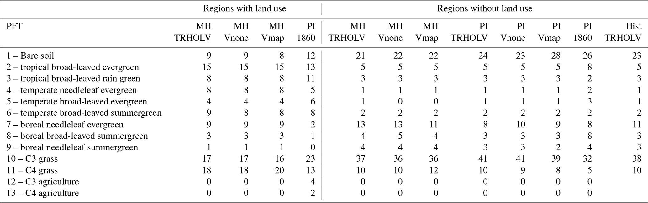
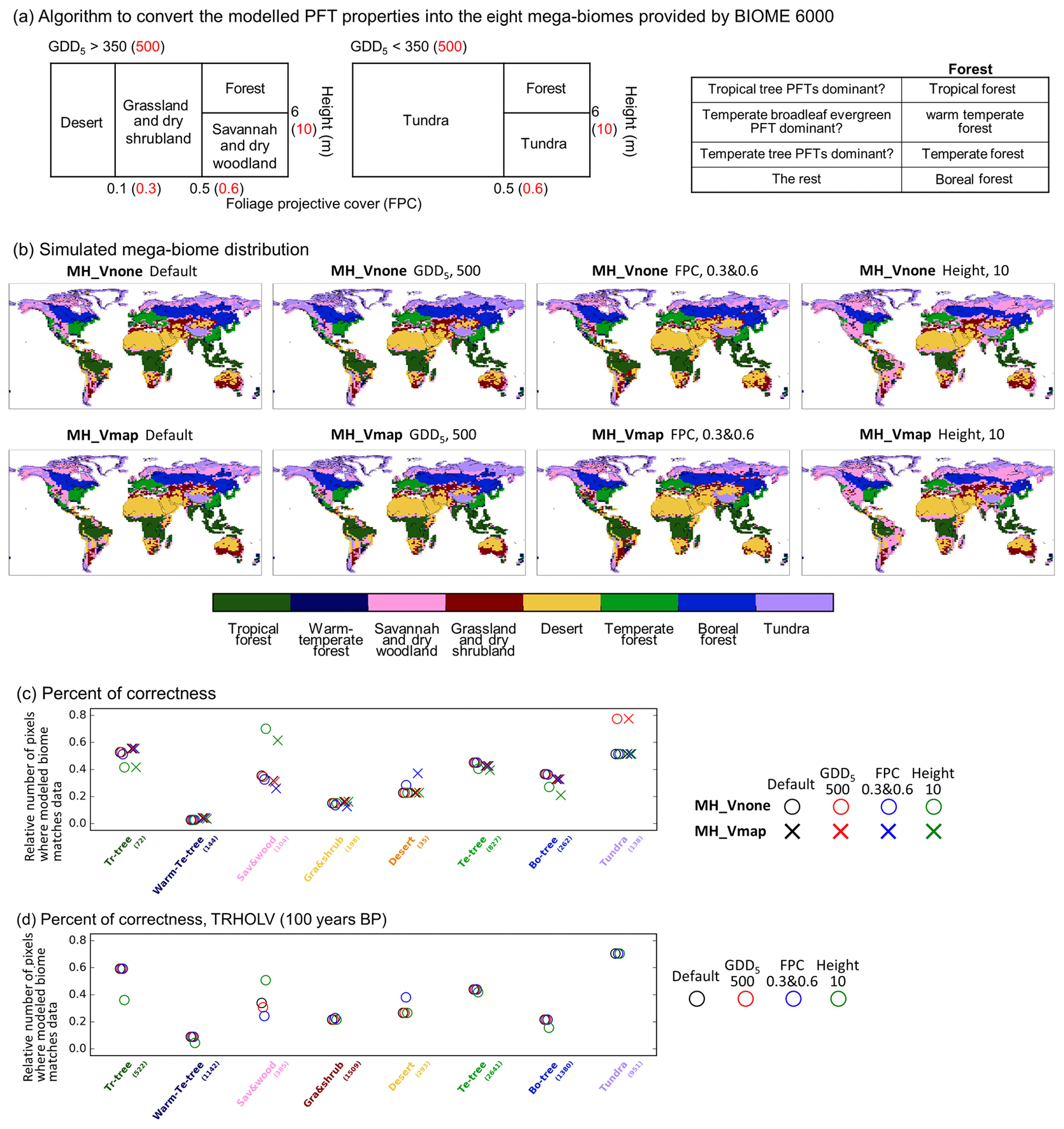
Figure A2(a) Algorithm to convert the modeled PFT properties into the eight mega-biomes provided by BIOME 6000 DB version 1. The default thresholds (in black) are the same as Zhu et al. (2018), while different values (in red) are tested: GDD5 (annual growing degree days above 5 ∘C) of 500 kelvin days (Joos et al., 2004), FPC (foliage projective cover) of 0.3 and 0.6 (Prentice et al., 2011), and height (average height of all existing tree PFTs) of 10 m (Prentice et al., 2011). (b) Simulated mega-biome distribution by MH_Vnone and MH_Vmap, using different conversion methods to (a). (c, d) The number of pixels where the modeled mega-biome matches data for each biome type, divided by the total number of available sites for that biome type, for the Mid-Holocene compared with BIOME 6000 6 ka (c) and for the preindustrial period compared with BIOME 6000 0 ka (d).
The different thresholds induce only a slight difference on the biome map for a given simulation. The largest sensitivity is obtained for the height. When 10 m is used instead of 6 m, a larger cover of savannah and dry woodland is estimated from the simulations in midlatitudes and high northern latitudes. In these latitudes also, a large sensitivity is found when the GDD5 limit is set to 500 ∘C d−1 instead of 350 ∘C d−1 between tundra and savannah and dry woodland or boreal forest.
The same analysis transformation into mega-biomes was performed for the Vmap and Vnone simulations. Similar sensitivity is found to the different thresholds for these two simulations (Fig. A2b). The synthesis of the goodness of fit between model and data is presented in Fig. A2c. It shows that, as expected, the two simulations provide very similar results when compared to the MH BIOME6000 map. It is interesting to note that the different thresholds do not have a large impact on the model–data comparison, when all data points are considered. The change in GDD5 limit produces tundra in better agreement with pollen data, and the canopy height produces better results with savannah and dry woodland. Note, however, that this result is in part due to the fact that there are few data in regions where the impact is the largest (Fig. 6 in the main text).
The same procedure was also applied to the PI Vnone and PI-Vmap simulations. The overall correctness (percentage of reconstruction sites showing the same mega-biome between model and data) is similar to the one obtained for MH (37 % for MH and 35 % for PI). These numbers are close to the percentages derived by Dallmeyer et al. (2019) using a climate-based biomization method (i.e., using Earth system model climate states to force a biogeography model to simulate the biome distribution), which gives 33 % and 39 % with two IPSL model versions for the preindustrial period.
PB and OM designed the experiments and prepared the model version. DZ ran the off-line simulations with the land surface model and performed the BIOME model–data comparison. PB ran the simulations. PB and OM analyzed the Holocene and the transient simulations and the relationship with the forcing. JS analyzed the model performances and provided the metrics. PB led the writing, and all co-authors contributed to the final version of the paper.
The authors declare that they have no conflict of interest.
We would like to thank our colleagues from the IPSL global climate model group for their help in setting up this intermediate version of the IPSL model. In particular, the ORCHIDEE group provided good advice for the closure of the hydrological cycle in the land surface scheme (Philippe Peylin, Agnès Ducharne, Fréderic Cheruy, and Joséfine Gattas) and the snow ablation (Sylvie Charbit and Christophe Dumas). The workflow for these long simulations benefits from the development of Anne Cozic and Arnaud Caubel. Discussions with Philippe Ciais and Yves Balkansky were also at the origin of the choice of the land surface model complexity and aerosols forcing strategy. We are grateful to the anonymous reviewers for their constructive comments that helped to improve the paper. We acknowledge PRACE for awarding us access to Curie at GENCI@CEA, France (THROL project) to start the simulations. The simulations were also performed using HPC resources from GENCI-TGCC thanks to a high-end computing access grant and to our annual allocation time (gen2212).
This research has been supported by the JPI-Belmont PACMEDY (grant no. ANR-15-JCLI-0003-01).
This paper was edited by Martin Claussen and reviewed by Anne Dallmeyer and one anonymous referee.
Abis, B. and Brovkin, V.: Environmental conditions for alternative tree-cover states in high latitudes, Biogeosciences, 14, 511–527, https://doi.org/10.5194/bg-14-511-2017, 2017.
Albani, S., Mahowald, N. M., Winckler, G., Anderson, R. F., Bradtmiller, L. I., Delmonte, B., François, R., Goman, M., Heavens, N. G., Hesse, P. P., Hovan, S. A., Kang, S. G., Kohfeld, K. E., Lu, H., Maggi, V., Mason, J. A., Mayewski, P. A., McGee, D., Miao, X., Otto-Bliesner, B. L., Perry, A. T., Pourmand, A., Roberts, H. M., Rosenbloom, N., Stevens, T., and Sun, J.: Twelves thousand years of dust: the Holocene global dust cycle constrained by natural archives, Clim. Past, 11, 869–903, https://doi.org/10.5194/cp-11-869-2015, 2015.
Alexandrov, D. V., Bashkirtseva, I. A., and Ryashko, L. B.: Noise-induced transitions and shifts in a climate–vegetation feedback model, Roy. Soc. Open Sci., 5, https://doi.org/10.1098/rsos.171531, 2018.
Aumont, O. and Bopp, L.: Globalizing results from ocean in situ iron fertilization studies, Global Biogeochemical Cy., 20, https://doi.org/10.1029/2005GB002591, 2006.
Bartlein, P. J., Harrison, S. P., Brewer, S., Connor, S., Davis, B. A. S., Gajewski, K., Guiot, J., Harrison-Prentice, T. I., Henderson, A., Peyron, O., Prentice, I. C., Scholze, M., Seppa, H., Shuman, B., Sugita, S., Thompson, R. S., Viau, A. E., Williams, J., and Wu, H.: Pollen-based continental climate reconstructions at 6 and 21 ka: a global synthesis, Clim. Dynam., 37, 775–802, 2011.
Bathiany, S., Claussen, M., and Fraedrich, K.: Implications of climate variability for the detection of multiple equilibria and for rapid transitions in the atmosphere-vegetation system, Clim. Dynam., 38, 1775–1790, 2012.
Berger, A.: Long-term variations of caloric solar radiation resulting from the Earth's orbital elements, Quaternary Res., 9, 139–167, 1978.
Bigelow, N. H., Brubaker, L. B., Edwards, M. E., Harrison, S. P., Prentice, I. C., Anderson, P. M., Andreev, A. A., Bartlein, P. J., Christensen, T. R., Cramer, W., Kaplan, J. O., Lozhkin, A. V., Matveyeva, N. V., Murray, D. F., McGuire, A. D., Razzhivin, V. Y., Ritchie, J. C., Smith, B., Walker, D. A., Gajewski, K., Wolf, V., Holmqvist, B. H., Igarashi, Y., Kremenetskii, K., Paus, A., Pisaric, M. F. J., and Volkova, V. S.: Climate change and Arctic ecosystems: 1. Vegetation changes north of 55 degrees N between the last glacial maximum, mid-Holocene, and present, J. Geophys. Res.-Atmos., 108, https://doi.org/10.1029/2002JD002558, 2003.
Boisier, J., Noblet-Ducoudré, N. d., Pitman, A., Cruz, F., Delire, C., den Hurk, B., Molen, M., Müller, C., and Voldoire, A.: Attributing the impacts of land–cover changes in temperate regions on surface temperature and heat fluxes to specific causes: Results from the first LUCID set of simulations, J. Geophys. Res.-Atmos., 117, https://doi.org/10.1029/2011JD017106, 2012.
Bonfils, C., de Noblet-Ducoure, N., Braconnot, P., and Joussaume, S.: Hot desert albedo and climate change: Mid-Holocene monsoon in North Africa, J. Climate, 14, 3724–3737, 2001.
Braconnot, P. and Kageyama, M.: Shortwave forcing and feedbacks in Last Glacial Maximum and Mid-Holocene PMIP3 simulations, Philos. Trans. R. Soc. A, 373, 20140424, https://doi.org/10.1098/rsta.2014.0424, 2015.
Braconnot, P., Marti, O., and Joussaume, S.: Adjustment and feedbacks in a global coupled ocean-atmosphere model, Clim. Dynam., 13, 507–519, 1997.
Braconnot, P., Joussaume, S., Marti, O., and de Noblet, N.: Synergistic feedbacks from ocean and vegetation on the African monsoon response to mid-Holocene insolation, Geophys. Res. Lett., 26, 2481–2484, 1999.
Braconnot, P., Otto-Bliesner, B., Harrison, S., Joussaume, S., Peterchmitt, J.-Y., Abe-Ouchi, A., Crucifix, M., Driesschaert, E., Fichefet, Th., Hewitt, C. D., Kageyama, M., Kitoh, A., Laîné, A., Loutre, M.-F., Marti, O., Merkel, U., Ramstein, G., Valdes, P., Weber, S. L., Yu, Y., and Zhao, Y.: Results of PMIP2 coupled simulations of the Mid-Holocene and Last Glacial Maximum – Part 1: experiments and large-scale features, Clim. Past, 3, 261–277, https://doi.org/10.5194/cp-3-261-2007, 2007a.
Braconnot, P., Otto-Bliesner, B., Harrison, S., Joussaume, S., Peterchmitt, J.-Y., Abe-Ouchi, A., Crucifix, M., Driesschaert, E., Fichefet, Th., Hewitt, C. D., Kageyama, M., Kitoh, A., Loutre, M.-F., Marti, O., Merkel, U., Ramstein, G., Valdes, P., Weber, L., Yu, Y., and Zhao, Y.: Results of PMIP2 coupled simulations of the Mid-Holocene and Last Glacial Maximum – Part 2: feedbacks with emphasis on the location of the ITCZ and mid- and high latitudes heat budget, Clim. Past, 3, 279–296, https://doi.org/10.5194/cp-3-279-2007, 2007b.
Braconnot, P., Harrison, S. P., Kageyama, M., Bartlein, P. J., Masson-Delmotte, V., Abe-Ouchi, A., Otto-Bliesner, B., and Zhao, Y.: Evaluation of climate models using palaeoclimatic data, Nat. Clim. Change, 2, 417–424, 2012.
Brovkin, V., Bendtsen, J., Claussen, M., Ganopolski, A., Kubatzki, C., Petoukhov, V., and Andreev, A.: Carbon cycle, vegetation, and climate dynamics in the Holocene: Experiments with the CLIMBER-2 model, Global Biogeochem. Cy., 16, https://doi.org/10.1029/2001GB001662, 2002.
Campbell, J. E., Berry, J. A., Seibt, U., Smith, S. J., Montzka, S. A., Launois, T., Belviso, S., Bopp, L., and Laine, M.: Large historical growth in global terrestrial gross primary production, Nature, 544, 84, https://doi.org/10.1038/nature22030, 2017.
Claussen, M.: Late Quaternary vegetation-climate feedbacks, Clim. Past, 5, 203–216, https://doi.org/10.5194/cp-5-203-2009, 2009.
Claussen, M. and Gayler, V.: The greening of the Sahara during the mid-Holocene: results of an interactive atmosphere-biome model, Global Ecol. Biogeogr., 6, 369–377, 1997.
COHMAP-Members: Climatic changes of the last 18 000 years: observations and model simulations, Science, 241, 1043–1052, 1988.
Crucifix, M., Loutre, M. F., Tulkens, P., Fichefet, T., and Berger, A.: Climate evolution during the Holocene: a study with an Earth system model of intermediate complexity, Clim. Dynam., 19, 43–60, 2002.
Dallmeyer, A., Claussen, M., and Otto, J.: Contribution of oceanic and vegetation feedbacks to Holocene climate change in monsoonal Asia, Clim. Past, 6, 195–218, https://doi.org/10.5194/cp-6-195-2010, 2010.
Dallmeyer, A., Claussen, M., and Brovkin, V.: Harmonising plant functional type distributions for evaluating Earth system models, Clim. Past, 15, 335–366, https://doi.org/10.5194/cp-15-335-2019, 2019.
Davis, B. A. S., Brewer, S., Stevenson, A. C., and Guiot, J.: The temperature of Europe during the Holocene reconstructed from pollen data, Quaternary Sci. Rev., 22, 1701–1716, 2003.
de Noblet, N., Prentice, I. C., Joussaume, S., Texier, D., Botta, A., and Haxeltine, A.: Possible role of atmosphere-biosphere interactions in triggering the last glaciation, Geophys. Res. Lett., 23, 3191–3194, 1996.
deMenocal, P., Ortiz, J., Guilderson, T., Adkins, J., Sarnthein, M., Baker, L., and Yarusinsky, M.: Abrupt onset and termination of the African Humid Period: rapid climate responses to gradual insolation forcing, Quaternary Sci. Rev., 19, 347–361, 2000.
de Noblet-Ducoudre, N., Claussen, R., and Prentice, C.: Mid-Holocene greening of the Sahara: first results of the GAIM 6000 year BP Experiment with two asynchronously coupled atmosphere/biome models, Clim. Dynam., 16, 643–659, 2000.
de Rosnay, P., Polcher, J., Bruen, M., and Laval, K.: Impact of a physically based soil water flow and soil-plant interaction representation for modeling large-scale land surface processes, J. Geophys. Res.-Atmos., 107, https://doi.org/10.1029/2001JD000634, 2002.
d'Orgeval, T., Polcher, J., and de Rosnay, P.: Sensitivity of the West African hydrological cycle in ORCHIDEE to infiltration processes, Hydrol. Earth Syst. Sci., 12, 1387–1401, https://doi.org/10.5194/hess-12-1387-2008, 2008.
Ducoudré, N., Laval, K., and Perrier, A.: SECHIBA, a new set of parameterizations of the hydrologic exchanges at the land/atmosphere interface within the LMD atmospheric general circulation model, J. Climate, 6, https://doi.org/10.1175/1520-0442(1993)006<0248:SANSOP>2.0.CO;2, 1993.
Dufresne, J. L., Foujols, M. A., Denvil, S., Caubel, A., Marti, O., Aumont, O., Balkanski, Y., Bekki, S., Bellenger, H., Benshila, R., Bony, S., Bopp, L., Braconnot, P., Brockmann, P., Cadule, P., Cheruy, F., Codron, F., Cozic, A., Cugnet, D., de Noblet, N., Duvel, J. P., Ethe, C., Fairhead, L., Fichefet, T., Flavoni, S., Friedlingstein, P., Grandpeix, J. Y., Guez, L., Guilyardi, E., Hauglustaine, D., Hourdin, F., Idelkadi, A., Ghattas, J., Joussaume, S., Kageyama, M., Krinner, G., Labetoulle, S., Lahellec, A., Lefebvre, M. P., Lefevre, F., Levy, C., Li, Z. X., Lloyd, J., Lott, F., Madec, G., Mancip, M., Marchand, M., Masson, S., Meurdesoif, Y., Mignot, J., Musat, I., Parouty, S., Polcher, J., Rio, C., Schulz, M., Swingedouw, D., Szopa, S., Talandier, C., Terray, P., Viovy, N., and Vuichard, N.: Climate change projections using the IPSL-CM5 Earth System Model: from CMIP3 to CMIP5, Clim. Dynam., 40, 2123–2165, 2013.
Egerer, S., Claussen, M., Reick, C., and Stanelle, T.: Could gradual changes in Holocene Saharan landscape have caused the observed abrupt shift in North Atlantic dust deposition?, Earth Planet. Sc. Lett., 473, 104–112, 2017.
Fichefet, T. and Maqueda, M. A. M.: Modelling the influence of snow accumulation and snow-ice formation on the seasonal cycle of the Antarctic sea-ice cover, Clim. Dynam., 15, 251–268, 1999.
Gleckler, P., Doutriaux, C., Durack, P., Taylor, K., Zhang, Y., Williams, D., Mason, E., and Servonnat, J.: A More Powerful Reality Test for Climate Models, EOS, Transactions of the American Geophysical Union, 97, https://doi.org/10.1029/2016EO051663, 2016.
Guimberteau, M., Zhu, D., Maignan, F., Huang, Y., Yue, C., Dantec-Nédélec, S., Ottlé, C., Jornet-Puig, A., Bastos, A., Laurent, P., Goll, D., Bowring, S., Chang, J., Guenet, B., Tifafi, M., Peng, S., Krinner, G., Ducharne, A., Wang, F., Wang, T., Wang, X., Wang, Y., Yin, Z., Lauerwald, R., Joetzjer, E., Qiu, C., Kim, H., and Ciais, P.: ORCHIDEE-MICT (v8.4.1), a land surface model for the high latitudes: model description and validation, Geosci. Model Dev., 11, 121–163, https://doi.org/10.5194/gmd-11-121-2018, 2018.
Harrison, S.: BIOME 6000 DB classified plotfile version 1, University of Reading, Dataset, available at: https://doi.org/10.17864/1947.99, 2017.
Harrison, S. P., Jolly, D., Laarif, F., Abe-Ouchi, A., Dong, B., Herterich, K., Hewitt, C., Joussaume, S., Kutzbach, J. E., Mitchell, J., de Noblet, N., and Valdes, P.: Intercomparison of Simulated Global Vegetation Distributions in Response to 6 kyr BP Orbital Forcing, J. Climate, 11, 2721–2742, 1998.
Harrison, S. P., Bartlein, P. J., Brewer, S., Prentice, I. C., Boyd, M., Hessler, I., Holmgren, K., Izumi, K., and Willis, K.: Climate model benchmarking with glacial and mid-Holocene climates, Clim. Dynam., 43, 671–688, 2014.
Held, I. M. and Soden, B. J.: Robust Responses of the Hydrological Cycle to Global Warming, J. Climate, 19, 5686–5699, 2006.
Hély, C., Lézine, A.-M., and contributors, A.: Holocene changes in African vegetation: tradeoff between climate and water availability, Clim. Past, 10, 681–686, https://doi.org/10.5194/cp-10-681-2014, 2014.
Hopcroft, P. O., Valdes, P. J., Harper, A. B., and Beerling, D. J.: Multi vegetation model evaluation of the Green Sahara climate regime, Geophys. Res. Lett., 44, 6804–6813, 2017.
Hourdin, F., Foujols, M. A., Codron, F., Guemas, V., Dufresne, J. L., Bony, S., Denvil, S., Guez, L., Lott, F., Ghattas, J., Braconnot, P., Marti, O., Meurdesoif, Y., and Bopp, L.: Impact of the LMDZ atmospheric grid configuration on the climate and sensitivity of the IPSL-CM5A coupled model, Clim. Dynam., 40, 2167–2192, 2013.
Jansen, E., Overpeck, J., Briffa, K. R., Duplessy, J. C., Joos, F., Masson-Delmotte, V., Olago, D., Otto-Bliesner, B., Peltier, W. R., Rahmstorf, S., Ramesh, R., Raynaud, D., Rind, D., Solomina, O., Villalba, R., and Zhang, D.: Paleoclimate, in: Climate Chane 2007: The Physical Science Basis. Contribution of Working Group I to the Fourth Assessement Report of the Intergovernmental Panel on Climate Change, edited by: Solomon, S., Qin, D. H., Manning, M., Chen, Z., Marsuis, M., Averyt, K. B., Tignor, M., and Miller, H. L., Cambridge University Press, Cambridge, UK and New York, NY, USA, 2007.
Jolly, D., Prentice, I. C., Bonnefille, R., Ballouche, A., Bengo, M., Brenac, P., Buchet, G., Burney, D., Cazet, J.-P., Cheddadi, R., Edohr, T., Elenga, H., Elmoutaki, S., Guiot, J., Laarif, F., Lamb, H., Lezine, A.-M., Maley, J., Mbenza, M., Peyron, O., Reille, M., Reynaud-Ferrera, I., Riollet, G., Ritchie, J. C., Roche, E., Scott, L., Ssemmanda, I., Straka, H., Umer, M., Van Campo, E., Vilimumbala, S., Vincens, A., and Waller, M.: Biome reconstruction from pollen and plant macrofossil data for Africa and the Arabian peninsula at 0 and 6 ka, J. Biogeogr., 25, 1007–1028, 1998.
Jomelli, V., Khodri, M., Favier, V., Brunstein, D., Ledru, M. P., Wagnon, P., Blard, P. H., Sicart, J. E., Braucher, R., Grancher, D., Bourles, D. L., Braconnot, P., and Vuille, M.: Irregular tropical glacier retreat over the Holocene epoch driven by progressive warming, Nature, 474, 196–199, 2011.
Joos, F. and Spahni, R.: Rates of change in natural and anthropogenic radiative forcing over the past 20 000 years, P. Natl. Acad. Sci. USA, 105, 1425–1430, 2008.
Joos, F., Gerber, S., Prentice, I., Otto-Bliesner, B., and Valdes, P.: Transient simulations of Holocene atmospheric carbon dioxide and terrestrial carbon since the Last Glacial Maximum, Global Biogeochem. Cy., 18, https://doi.org/10.1029/2003GB002156, 2004.
Joussaume, S. and Braconnot, P.: Sensitivity of paleoclimate simulation results to season definitions, J. Geophys. Res., 102, 1943–1956, 1997.
Joussaume, S., Taylor, K. E., Braconnot, P., Mitchell, J. F. B., Kutzbach, J. E., Harrison, S. P., Prentice, I. C., Broccoli, A. J., Abe-Ouchi, A., Bartlein, P. J., Bonfils, C., Dong, B., Guiot, J., Herterich, K., Hewitt, C. D., Jolly, D., Kim, J. W., Kislov, A., Kitoh, A., Loutre, M. F., Masson, V., McAvaney, B., McFarlane, N., de Noblet, N., Peltier, W. R., Peterschmitt, J. Y., Pollard, D., Rind, D., Royer, J. F., Schlesinger, M. E., Syktus, J., Thompson, S., Valdes, P., Vettoretti, G., Webb, R. S., and Wyputta, U.: Monsoon changes for 6000 years ago: Results of 18 simulations from the Paleoclimate Modeling Intercomparison Project (PMIP), Geophys. Res. Lett., 26, 859–862, 1999.
Kageyama, M., Braconnot, P., Bopp, L., Caubel, A., Foujols, M. A., Guilyardi, E., Khodri, M., Lloyd, J., Lombard, F., Mariotti, V., Marti, O., Roy, T., and Woillez, M. N.: Mid-Holocene and Last Glacial Maximum climate simulations with the IPSL model-part I: comparing IPSL_CM5A to IPSL_CM4, Clim. Dynam., 40, 2447–2468, 2013a.
Kageyama, M., Braconnot, P., Bopp, L., Mariotti, V., Roy, T., Woillez, M. N., Caubel, A., Foujols, M. A., Guilyardi, E., Khodri, M., Lloyd, J., Lombard, F., and Marti, O.: Mid-Holocene and last glacial maximum climate simulations with the IPSL model: part II: model-data comparisons, Clim. Dynam., 40, 2469–2495, 2013b.
Kageyama, M., Braconnot, P., Harrison, S. P., Haywood, A. M., Jungclaus, J. H., Otto-Bliesner, B. L., Peterschmitt, J.-Y., Abe-Ouchi, A., Albani, S., Bartlein, P. J., Brierley, C., Crucifix, M., Dolan, A., Fernandez-Donado, L., Fischer, H., Hopcroft, P. O., Ivanovic, R. F., Lambert, F., Lunt, D. J., Mahowald, N. M., Peltier, W. R., Phipps, S. J., Roche, D. M., Schmidt, G. A., Tarasov, L., Valdes, P. J., Zhang, Q., and Zhou, T.: The PMIP4 contribution to CMIP6 – Part 1: Overview and over-arching analysis plan, Geosci. Model Dev., 11, 1033–1057, https://doi.org/10.5194/gmd-11-1033-2018, 2018.
Krinner, G., Viovy, N., de Noblet-Ducoudre, N., Ogee, J., Polcher, J., Friedlingstein, P., Ciais, P., Sitch, S., and Prentice, I. C.: A dynamic global vegetation model for studies of the coupled atmosphere-biosphere system, Global Biogeochem. Cy., 19, https://doi.org/10.1029/2003GB002199, 2005.
Kutzbach, J. E., Bartlein, P. J., Foley, J. A., Harrison, S. P., Hostetler, S. W., Liu, Z., Prentice, I. C., and Webb, T.: Potential role of vegetation feedback in the climate sensitivity of high-latitude regions: A case study at 6000 years BP, Global Biogeochem. Cy., 10, 727–736, 1996.
Lenton, T. M., Held, H., Kriegler, E., Hall, J. W., Lucht, W., Rahmstorf, S., and Schellnhuber, H. J.: Tipping elements in the Earth's climate system, P. Natl. Acad. Sci. USA, 105, 1786-1793, 2008.
Levis, S., Bonan, G. B., and Bonfils, C.: Soil feedback drives the mid-Holocene North African monsoon northward in fully coupled CCSM2 simulations with a dynamic vegetation model, Clim. Dynam., 23, 791–802, 2004.
Lezine, A. M., Hely, C., Grenier, C., Braconnot, P., and Krinner, G.: Sahara and Sahel vulnerability to climate changes, lessons from Holocene hydrological data, Quaternary Sci. Rev., 30, 3001–3012, 2011.
Lezine, A. M., Ivory, S. J., Braconnot, P., and Marti, O.: Timing of the southward retreat of the ITCZ at the end of the Holocene Humid Period in Southern Arabia: Data-model comparison, Quaternary Sci. Rev., 164, 68–76, 2017.
Liu, Z., Wang, Y., Gallimore, R., Gasse, F., Johnson, T., deMenocal, P., Adkins, J., Notaro, M., Prenticer, I. C., Kutzbach, J., Jacob, R., Behling, P., Wang, L., and Ong, E.: Simulating the transient evolution and abrupt change of Northern Africa atmosphere-ocean-terrestrial ecosystem in the Holocene, Quaternary Sci. Rev., 26, 1818–1837, 2007.
Liu, Z. Y., Zhu, J., Rosenthal, Y., Zhang, X., Otto-Bliesner, B. L., Timmermann, A., Smith, R. S., Lohmann, G., Zheng, W. P., and Timm, O. E.: The Holocene temperature conundrum, P. Natl. Acad. Sci. USA, 111, E3501–E3505, 2014.
Madec, G.: NEMO ocean engine, available at: https://www.nemo-ocean.eu/doc/ (last access: 3 June 2019), 2008.
Marsicek, J., Shuman, B. N., Bartlein, P. J., Shafer, S. L., and Brewer, S.: Reconciling divergent trends and millennial variations in Holocene temperatures, Nature, 554, 92, https://doi.org/10.1038/nature25464, 2018.
Marti, O., Braconnot, P., Dufresne, J. L., Bellier, J., Benshila, R., Bony, S., Brockmann, P., Cadule, P., Caubel, A., Codron, F., de Noblet, N., Denvil, S., Fairhead, L., Fichefet, T., Foujols, M. A., Friedlingstein, P., Goosse, H., Grandpeix, J. Y., Guilyardi, E., Hourdin, F., Idelkadi, A., Kageyama, M., Krinner, G., Levy, C., Madec, G., Mignot, J., Musat, I., Swingedouw, D., and Talandier, C.: Key features of the IPSL ocean atmosphere model and its sensitivity to atmospheric resolution, Clim. Dynam., 34, 1–26, 2010.
Mauri, A., Davis, B., Collins, P., and Kaplan, J.: The climate of Europe during the Holocene: a gridded pollen-based reconstruction and its multi-proxy evaluation, Quaternary Sci. Rev., 112, 109–127, 2015.
Otto, J., Raddatz, T., Claussen, M., Brovkin, V., and Gayler, V.: Separation of atmosphere-ocean-vegetation feedbacks and synergies for mid-Holocene climate, Geophys. Res. Lett., 36, https://doi.org/10.1029/2009GL037482, 2009.
Otto, J., Raddatz, T., and Claussen, M.: Strength of forest-albedo feedback in mid-Holocene climate simulations, Clim. Past, 7, 1027–1039, https://doi.org/10.5194/cp-7-1027-2011, 2011.
Otto-Bliesner, B. L., Braconnot, P., Harrison, S. P., Lunt, D. J., Abe-Ouchi, A., Albani, S., Bartlein, P. J., Capron, E., Carlson, A. E., Dutton, A., Fischer, H., Goelzer, H., Govin, A., Haywood, A., Joos, F., LeGrande, A. N., Lipscomb, W. H., Lohmann, G., Mahowald, N., Nehrbass-Ahles, C., Pausata, F. S. R., Peterschmitt, J.-Y., Phipps, S. J., Renssen, H., and Zhang, Q.: The PMIP4 contribution to CMIP6 – Part 2: Two interglacials, scientific objective and experimental design for Holocene and Last Interglacial simulations, Geosci. Model Dev., 10, 3979–4003, https://doi.org/10.5194/gmd-10-3979-2017, 2017.
Pausata, F. S., Messori, G., and Zhang, Q.: Impacts of dust reduction on the northward expansion of the African monsoon during the Green Sahara period, Earth Planet. Sc. Lett., 434, 298–307, 2016.
Prentice, I. C. and Webb, T.: BIOME 6000: reconstructing global mid-Holocene vegetation patterns from palaeoecological records, J. Biogeogr., 25, 997–1005, 1998.
Prentice, I. C., Harrison, S. P., and Bartlein, P. J.: Global vegetation and terrestrial carbon cycle changes after the last ice age, New Phytol., 189, 988–998, 2011.
Renssen, H., Seppä, H., Crosta, X., Goosse, H., and Roche, D. M.: Global characterization of the Holocene Thermal Maximum, Quaternary Sci. Rev., 48, 7–19, 2012.
Saint-Lu, M., Braconnot, P., Leloup, J., and Marti, O.: The role of El Niño in the global energy redistribution: a case study in the mid-Holocene, Clim. Dynam., 2016, 1–18, 2016.
Scheffer, M., Hirota, M., Holmgren, M., Van Nes, E. H., and Chapin, F. S.: Thresholds for boreal biome transitions, P. Natl. Acad. Sci. USA, 109, 21384–21389, 2012.
Singarayer, J. S. and Valdes, P. J.: High-latitude climate sensitivity to ice-sheet forcing over the last 120 kyr, Quaternary Sci. Rev., 29, 43–55, 2010.
Texier, D., de Noblet, N., Harrison, S. P., Haxeltine, A., Jolly, D., Joussaume, S., Laarif, F., Prentice, I. C., and Tarasov, P.: Quantifying the role of biosphere-atmosphere feedbacks in climate change: coupled model simulations for 6000 years BP and comparison with palaeodata for northern Eurasia and northern Africa, Clim. Dynam., 13, 865–882, 1997.
Torres, O., Braconnot, P., Marti, O., and Gential, L.: Impact of air-sea drag coefficient for latent heat flux on large scale climate in coupled and atmosphere stand-alone simulations, Clim. Dynam., 2018, 1–20, 2018.
Valcke, S.: OASIS3 user's guide (prism-2-5), CERFACS, Toulouse, France, 2006.
Vial, J., Dufresne, J. L., and Bony, S.: On the interpretation of inter-model spread in CMIP5 climate sensitivity estimates, Clim. Dynam., 41, 3339–3362, 2013.
Wang, T., Ottlé, C., Boone, A., Ciais, P., Brun, E., Morin, S., Krinner, G., Piao, S., and Peng, S.: Evaluation of an improved intermediate complexity snow scheme in the ORCHIDEE land surface model, J. Geophys. Res.-Atmos., 118, 6064–6079, 2013.
Wanner, H., Beer, J., Buetikofer, J., Crowley, T. J., Cubasch, U., Flueckiger, J., Goosse, H., Grosjean, M., Joos, F., Kaplan, J. O., Kuettel, M., Mueller, S. A., Prentice, I. C., Solomina, O., Stocker, T. F., Tarasov, P., Wagner, M., and Widmann, M.: Mid- to Late Holocene climate change: an overview, Quaternary Sci. Rev., 27, 1791–1828, 2008.
Wohlfahrt, J., Harrison, S. P., and Braconnot, P.: Synergistic feedbacks between ocean and vegetation on mid- and high-latitude climates during the mid-Holocene, Clim. Dynam., 22, 223–238, 2004.
Woillez, M.-N., Kageyama, M., Krinner, G., de Noblet-Ducoudré, N., Viovy, N., and Mancip, M.: Impact of CO2 and climate on the Last Glacial Maximum vegetation: results from the ORCHIDEE/IPSL models, Clim. Past, 7, 557–577, https://doi.org/10.5194/cp-7-557-2011, 2011.
Zhu, D., Peng, S. S., Ciais, P., Viovy, N., Druel, A., Kageyama, M., Krinner, G., Peylin, P., Ottlé, C., Piao, S. L., Poulter, B., Schepaschenko, D., and Shvidenko, A.: Improving the dynamics of Northern Hemisphere high-latitude vegetation in the ORCHIDEE ecosystem model, Geosci. Model Dev., 8, 2263–2283, https://doi.org/10.5194/gmd-8-2263-2015, 2015.
Zhu, D., Ciais, P., Chang, J., Krinner, G., Peng, S., Viovy, N., Peñuelas, J., and Zimov, S.: The large mean body size of mammalian herbivores explains the productivity paradox during the Last Glacial Maximum, Nature Ecology & Evolution, 2, 640–649, 2018.
- Abstract
- Introduction
- Model and the suite of experiments
- Simulated climate and vegetation throughout the Mid- to Late Holocene
- Vegetation, uncertainties, and multiple vegetation states
- Conclusion
- Data availability
- Appendix A: Spatiotemporal agreement between model results and observations in the extratropics and tropics
- Author contributions
- Competing interests
- Acknowledgements
- Financial support
- Review statement
- References