the Creative Commons Attribution 4.0 License.
the Creative Commons Attribution 4.0 License.
 | 02 Jun 2020
The mechanism of sapropel formation in the Mediterranean Sea: insight from long-duration box model experiments
Paul Meijer
Periodic bottom-water oxygen deficiency in the Mediterranean Sea led to the deposition of organic-rich sediments during geological history, so-called sapropels. Although a mechanism linking the formation of these deposits to orbital variability has been derived from the geological record, physics-based proof is limited to snapshot and short-time-slice experiments with (oceanic) general circulation models. Specifically, previous modelling studies have investigated atmospheric and oceanographic equilibrium states during orbital extremes (minimum and maximum precession). In contrast, we use a conceptual box model that allows us to focus on the transient response of the Mediterranean Sea to orbital forcing and investigate the physical processes causing sapropel formation. The model is constrained by present-day measurement data, while proxy data offer constraints on the timing of sapropels.
The results demonstrate that it is possible to describe the first-order aspects of sapropel formation in a conceptual box model. A systematic model analysis provides new insights on features observed in the geological record, such as the timing of sapropels as well as intra-sapropel intensity variations and interruptions. Moreover, given a scenario constrained by geological data, the model allows us to study the transient response of variables and processes that cannot be observed in the geological record. The results suggest that atmospheric temperature variability plays a key role in sapropel formation and that the timing of the midpoint of a sapropel can shift significantly with a minor change in forcing due to nonlinearities in the system.


1.1 Background
The response of ocean circulation to changes in atmospheric forcing is an important element of the climate system. Using computer models applied to the geological past, we can exploit the sedimentary record of variation in circulation for mechanistic insight. The Mediterranean Sea is of particular interest, as abundant and exceptionally well-dated proxy data and present-day measurement data are available, and it is a basin that displays processes such as thermohaline circulation and gateway control that play a role on the global scale as well.
Presently, the Mediterranean Sea is an evaporative basin (Romanou et al., 2010) with a small annual mean heat loss to the atmosphere (Song and Yu, 2017). Water from the Atlantic flows in to the Mediterranean Sea at the Strait of Gibraltar and is then subjected to buoyancy loss due to evaporation and cooling (see Fig. 1 for a map of the Mediterranean Sea). This results in the formation of intermediate water in the Levantine basin which spreads throughout the basin (Hayes et al., 2019; Wu and Haines, 1996). During winter, in the northerly parts of the basin situated at relatively high latitude, cold and dry winds induce a further density increase, which may lead to the formation of deep water (Schroeder et al., 2012). Specifically, deepwater formation (DWF) occurs over the shallow northern Adriatic Sea (Malanotte-Rizzoli, 1991), the Aegean Sea (Gertman et al., 2006; Roether et al., 1996), and in the form of open-ocean deep convection in the Gulf of Lion (Marshall and Schott, 1999) and the southern Adriatic Sea (Bensi et al., 2013). Dense water formed in the Adriatic and Aegean seas, both marginal basins of the Mediterranean Sea, flows out over the sea floor into the deeper parts of the main basin.
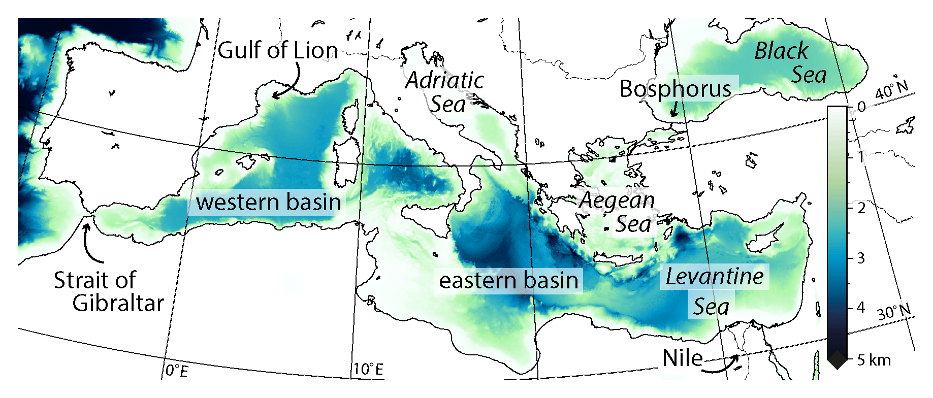
Figure 1Map of the Mediterranean Sea. The bathymetry shown is part of the GEBCO 2014 grid. The colours indicate water depth.
The basin's semi-enclosed nature causes the system to be very sensitive to climatic perturbations, and the geological record holds an expression of this sensitivity in the form of the regular occurrence of organic-rich deposits known as sapropels (Rossignol-Strick, 1985; Rohling et al., 2015; Hilgen, 1991; Lourens et al., 1996; Cramp and O'Sullivan, 1999). Sapropels are thought to form when Nile discharge increases as a response to enhanced African summer monsoon activity during precession minima (Rossignol-Strick, 1985; Rohling et al., 2015). The low-density fresh water then forms a lid at the surface, stopping or reducing the strength of the overturning circulation. This commonly accepted mechanism can be nuanced by noting that the Nile does not enter the basin at a DWF site, but rather close to the location where intermediate water forms. A large part of DWF involves this intermediate water (Schroeder et al., 2012). Reducing the density of the intermediate water implies a decrease in or the absence of a (positive) vertical density gradient, also diminishing or stopping the formation of deep water. In contrast, runoff into the marginal basins directly affects the buoyancy at DWF sites. For deep convection in, for example, the Levantine basin (which can happen with present-day conditions; Gertmann et al., 1994) a decrease in surface water density directly decreases or stops DWF. With decreasing DWF, the supply of oxygen to the deep water diminishes, potentially causing anoxia and the preservation of organic matter in the eastern Mediterranean Sea. Moreover, nutrient input increases with river outflow as well, thereby affecting primary production, the export of organic carbon to the deep water and, consequently, oxygen consumption (Calvert et al., 1992; De Lange and Ten Haven, 1983; Thomson et al., 1999; van Helmond et al., 2015; Weldeab et al., 2003). Sea level rise may also trigger sapropel formation (see Rohling et al., 2015, for sapropel S1), although this does not exclude monsoon intensity variability as the main cause.
In this paper we present a simple three-box model of the Mediterranean Sea, which includes most elements commonly invoked to explain sapropel formation as described above. With the model we study which processes determine when and why sapropels form the way they do. Our aim is to gain a new perspective on the timing of the sapropel relative to the forcing, as a significant part of the geological timescale depends on this relation (Hilgen et al., 1995; Krijgsman et al., 1999) and views on the timing of the midpoint (the average of the top and bottom age) are contested in more recent publications (Channell et al., 2010; Westerhold et al., 2012, 2015). A low-complexity model allows us to perform many long runs and explore the parameter space to a much greater extent than high-complexity models. The runs described in this paper represent but a small fraction of the experiments that have been conducted and were chosen to give an overview of the behaviour of the model. Long runs are necessary to study the transient response of the system over a full precession cycle.
As described in modelling studies (such as Marzocchi et al., 2015) and in observational studies (for example Herbert et al., 2015), surface air temperatures have also been found to vary over a precession cycle, wherein precession minima are estimated to have been 1–3 ∘C warmer (annual average) than precession maxima. Since heat loss depends on the temperature difference between the water surface and the atmosphere, this is another factor that decreases buoyancy loss during precession minima. We will examine the relative importance of this effect by running the model both with and without atmospheric temperature variability.
1.2 Previous modelling studies
Just like the Last Glacial Maximum, the time of sapropel formation was recognized early on in the application of OGCMs to Mediterranean circulation as a configuration that makes for an interesting contrast to the present-day state (Bigg, 1994; Myers et al., 1998; Myers and Rohling, 2000; Myers, 2002; Meijer and Tuenter, 2007; Meijer and Dijkstra, 2009) and, more recently, using a regional ocean model forced by output from a dedicated global climate model experiment (Mikolajewicz, 2011; Adloff et al., 2011). Several studies have explored the coupling of circulation models to models of the biogeochemical cycling, first offline and then in truly combined fashion (Stratford et al., 2000; Bianchi et al., 2006; Grimm et al., 2015). All these studies have in common that they are limited to time spans much shorter than the precessional cycle. The only previous box models related to the sapropel problem are those by Matthiesen and Haines (2003) and Amies et al. (2019), but these models lacks a representation of the deep waters of the basin.
The aforementioned studies offer support for the basic idea that freshening of the surface waters leads to reduction of the overturning circulation. The studies suggest that it is important to consider the full freshwater budget and that runoff may have varied significantly on orbital timescales (Bigg, 1994; Amies et al., 2019). Finally, nutrient supply is found be a significant factor in the formation of sapropels (Stratford et al., 2000; Bianchi et al., 2006).
2.1 Model set-up
The Mediterranean Sea is represented by three boxes in our model: the high-latitude marginal basins (intermediate and surface water, box 1, representing the Adriatic and Aegean seas and the Gulf of Lion), the open Mediterranean (surface and intermediate water, box 2) and the deep water (box 3) (see Fig. 2). Boxes 1 and 2 have fluvial input (sourced from boxes R1 and R2; see Fig. 2) and exchange with the atmosphere (represented by boxes A1 and A2; see Fig. 2). The surface forcing is further explained in Sect. 2.2. Each box has its own temperature and salinity. Boxes 1 through 3 are dynamic: the temperature, salinity and density are calculated during each time step based on the incoming and outgoing salt and heat. The Atlantic, both rivers and both parts of the atmosphere can be seen as static boxes: their salinity, temperature and density are constant.
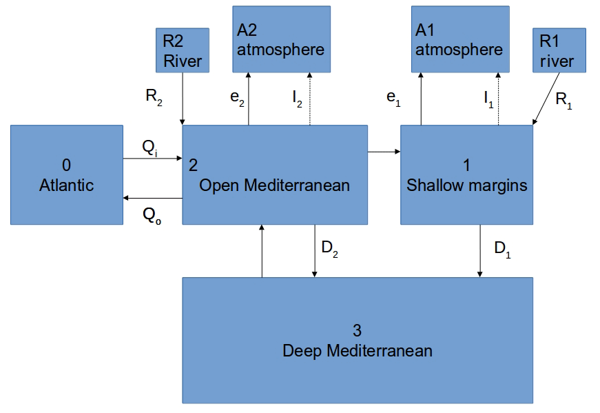
Figure 2A schematic overview of the model set-up. The unlabelled fluxes are balancing fluxes, and the equations for all fluxes are given in Sect. 2.3. The direction of the arrows indicates the positive direction in the equations; all horizontal fluxes can change direction.
Circulation is modelled by including downward vertical fluxes, the magnitude of which depends on the density difference between the surface–intermediate layer and the deep water (D1 in box 1 and D2 in box 2 in Fig. 2). This DWF is driven by buoyancy loss due to net evaporation (E–P, where E is the evaporation and P precipitation; e1 and e2 in Fig. 2) and heat exchange with the atmosphere, which is modelled as a relaxation (i.e. the surface water temperature relaxes to the temperature of the associated atmosphere box; fluxes I1 and I2 in Fig. 2). Note that the DWF in box 1 captures the behaviour of the marginal basins of the eastern Mediterranean Sea but is also an approximation of the open-ocean convection in the Gulf of Lion (see Sect. 1.1). In the typical situation that the Mediterranean surface–intermediate water at the Strait of Gibraltar is more dense than the Atlantic water and E–P–R (the freshwater budget, wherein R is the total runoff) is positive, it is the outflow to the Atlantic (Qo in Fig. 2) that depends on the density difference between the adjacent water masses. The inflow into the Mediterranean Sea is then the sum of the outflow to the Atlantic and the freshwater budget. The equations used in the model are further explained in Sect. 2.3.
In addition to the water fluxes, diffusive mixing is also included in the model. In contrast to the water fluxes, no net water transport occurs as a result of the mixing. Rather, properties are exchanged between adjacent boxes. The amount of horizontal mixing (between the upper boxes) is constant, while the vertical mixing is a function of the density difference between the boxes in question.
A first-order approximation of deepwater oxygen concentration is included in the model to get a better understanding of when oxygen deficiency occurs. The oxygen concentration of the upper boxes is assumed to be in equilibrium with the atmosphere and is therefore constant. The oxygen concentration of the deep water (box 3) depends on the deepwater fluxes, mixing and oxygen consumption. Oxygen consumption is scaled with river outflow, as a first-order approximation of the nutrient input, and oxygen concentration.
The use of constant volume for the boxes implies (i) that we take there to always be a distinction between surface–intermediate and deep cells, and (ii) the upper cell always extends to the same depth. The upper cell appears to be set up by the exchange with the ocean (see Meijer and Dijkstra, 2009, for the Mediterranean Sea and Finnigan et al., 2001, for a generic buoyancy-driven marginal sea) and is likely a persistent feature of Mediterranean circulation as long as there is an exchange flow. Moreover, starting from a state that does have DWF and a separate deep cell, OGCM experiments of reduced net evaporation show a halting of deep circulation while keeping the upper cell more or less in place (Meijer and Dijkstra, 2009).
In the present-day Mediterranean Sea DWF is the last step in a chain of processes (see the Introduction). Our model does not include intra-annual variability, and the basin geometry is only represented in abstract form. However, in the sense that the model does capture both the effect of salinity increase and temperature decrease on upper-water density it is expected to form a fair representation, qualitatively speaking, of the essence of the overturning circulation. To what extent this is true will have to follow from more advanced models. Note that the model of Matthiesen and Haines (2003) also neglects the seasonal cycle. During winter, convection occurs (Schroeder et al., 2012) and the depth of the intermediate water is relatively stable. We therefore abstract the circulation to an open surface–intermediate box, a marginal surface–intermediate box and a deepwater box, all with constant volumes. While the formation of deep water itself is a seasonal process, we parameterize the seasonal variability by calculating an annually averaged DWF flux. We know that DWF occurs every year during present winters. However, deep water would not form with annual average conditions and therefore we assume perpetual winter conditions.
2.2 Surface forcing
The transient response of circulation and water properties to precession-induced climate change is modelled by altering the evaporation and river outflow for each box at every time step. The analyses presented in this paper all use sine waves to force the model, but any temporal variation could be used, such as that of the insolation curve. To be precise, the model forcing used in this paper is derived from a normalized sine wave with a 20 kyr period to reflect climatic precession. The amplitude and offset are then altered for evaporation and fluvial discharge in boxes 1 and 2. The phase of evaporation relative to the precession forcing is uncertain (see Sect. 3.4) and is therefore varied between runs; the phase of the river discharge is kept at 0∘.
The fluvial discharge in box 2 (R2) is interpreted as Nile outflow and other runoff from Africa. Prior to the construction of the Aswan High Dam in 1964, average Nile discharge was 2.7×10³ m3 s−1 (Rohling et al., 2015). Present-day runoff from Africa is approximately 1.4×10³ m3 s−1 (Struglia et al., 2004). A recent modelling study (Amies et al., 2019) suggests that peak runoff from Africa may have been up to 8.8 times larger than present during sapropel S5. Note that the Amies et al. (2019) study does not consider changes in outflow from Europe.
Fluvial discharge into the high-latitude marginal basins of the Mediterranean Sea (R1 in the model) is presently approximately 6.7×10³ m3 s−1 (Struglia et al., 2004). Increased runoff from Europe into the eastern Mediterranean has been proposed as a possible source for extra fresh water during precession minima (Rossignol-Strick, 1985; Rohling et al., 2002; Scrivner et al., 2004)
The current net evaporation (E–P) is approximately 0.9 m yr−1 (Romanou et al., 2010). During sapropel times, net evaporation is hypothesized to have decreased (Rohling, 1994), although this has not been quantified. We therefore test a broad range of net evaporation from 0.2 to 2 m yr−1 to accommodate these uncertainties.
2.3 Model equations and parameters
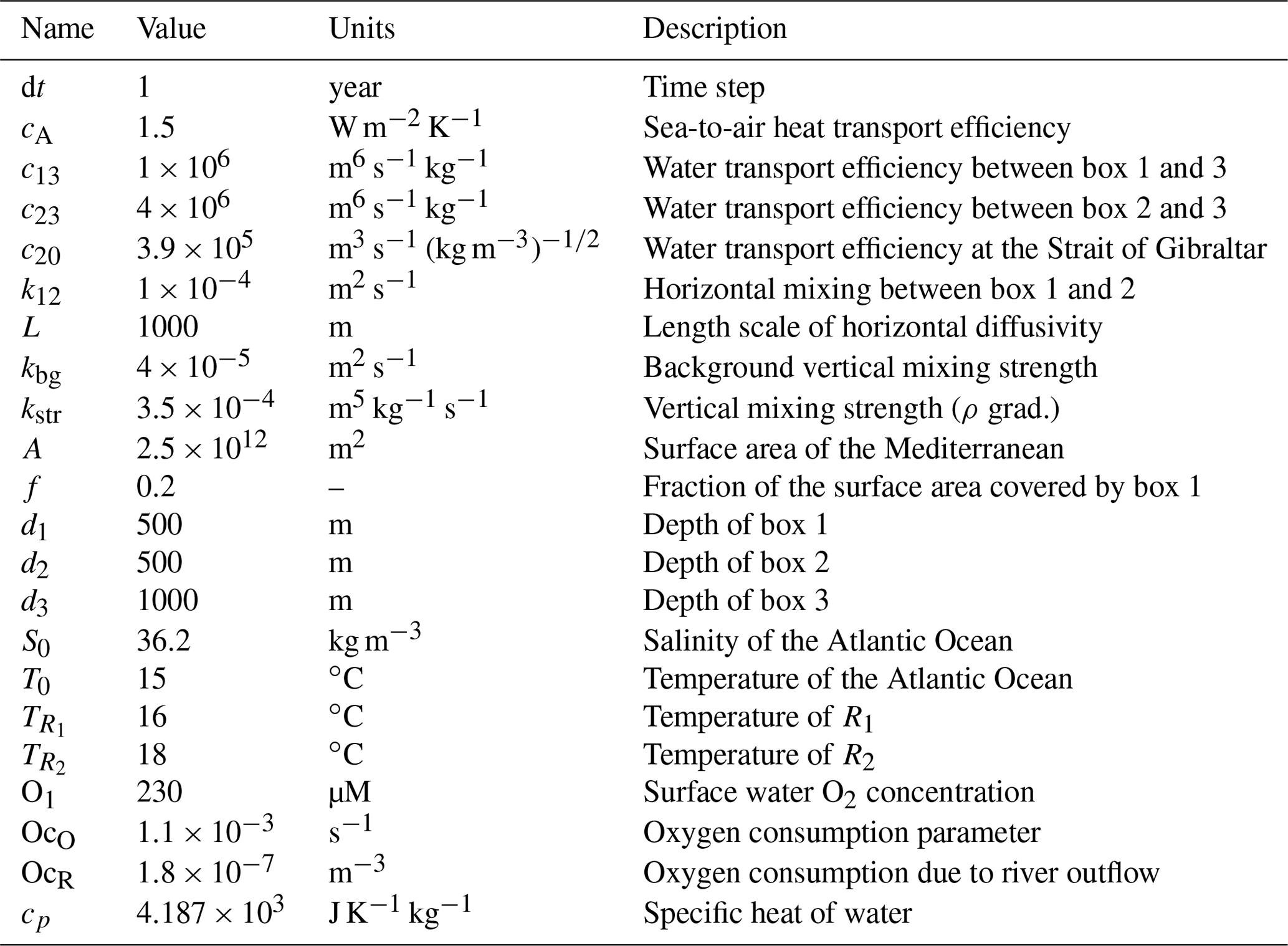
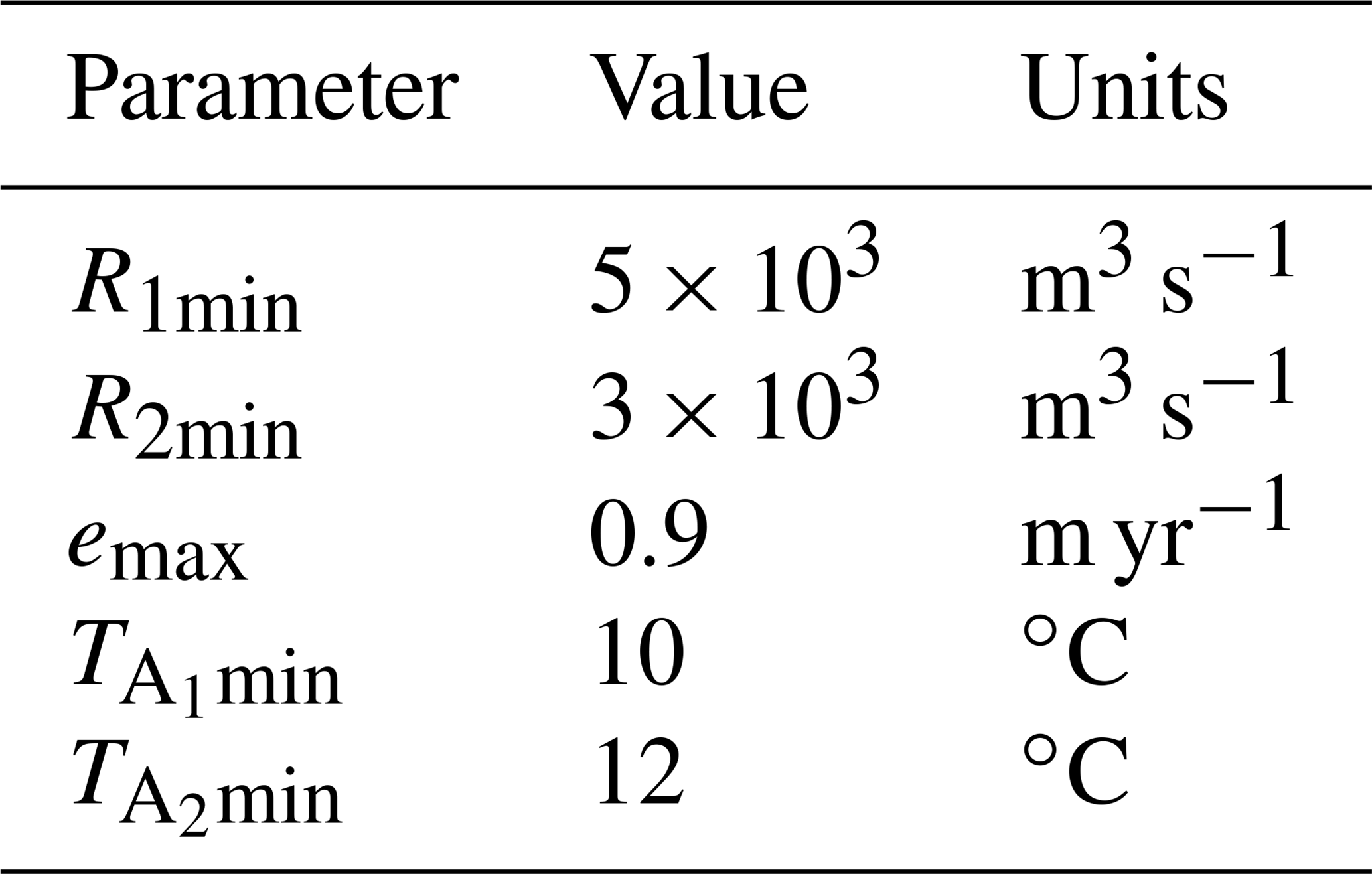
Here we first discuss the flux equations resulting from the model set-up and the assumptions described above, followed by the equations used to integrate all flux equations into a fully functioning model. All parameters are given in Table 1. We use a matrix–vector representation to calculate the temperatures, salinities, densities and oxygen concentration of the next time step. The (water and heat) flux magnitudes and mixing intensities define the elements of the matrices used for these calculations. This same matrix–vector representation could be used for an arbitrary configuration (and number) of boxes to represent different oceanographic settings.
Observational and modelling studies (Herrmann et al., 2008; Schroeder et al., 2012) have shown that during colder winters, more deep water is formed. Hence, it makes sense that the magnitude of the vertical downward fluxes (D1 and D2; see Eqs. 2 and 3) depends on oceanographic (and thereby indirectly also atmospheric) conditions. The most simple way of implementing this behaviour on a yearly resolution is to assume a linear relationship between the density difference and flux magnitude (similar to Matthiesen and Haines, 2003). When the density of the overlying water mass is smaller than that of the deep water, the water column is stratified and no vertical flux exists. To clip negative components of a flux to 0, we use the form , where a is the flux in question. We therefore define the following mathematical operator.
The proportionality of DWF to surface to deepwater density difference is determined by an efficiency constant, c13 and c23 for D1 and D2, respectively. The magnitude of these constants is chosen in such a way that a realistic deepwater flux occurs at a present-day density difference. In the current circulation deep convection in the Levantine basin (represented by D2) does not occur every year (Gertman et al., 1994; Pinardi et al., 2015), making it difficult to determine c23 empirically. By assuming that the DWF process in box 2 is the same as in box 1 (i.e. linearly dependent on the vertical density difference), c23 can be taken as 4 times larger than c13, proportional to the difference in the surface area of boxes 1 and 2. We therefore define the DWF fluxes in Eqs. (2) and (3), where ρ1, ρ2 and ρ3 are the densities of boxes 1 to 3, respectively.
At the Strait of Gibraltar, the exchange has two components from which the inflow and outflow are calculated (see equations below): a density-driven flux Qo (Eq. 4) and a compensating flux Qi (Eq. 5). The magnitude of Qo has a square root relation to the horizontal density difference at the strait (where ρ0 is the density of the Atlantic Ocean), in accordance with Bryden and Kinder (1991). Theoretically, this flux should be able to change direction when the density difference changes sign. We therefore multiply the square root of the absolute value of the density difference with the sign of the density difference. Note that the direction of the fluxes (i.e. whether it goes in or out of the Mediterranean Sea) is determined in Eqs. (11) and (10). The strait efficiency c20 (the coefficient of proportionality between volume transport and density difference) is again calibrated on present-day conditions (Schroeder et al., 2012; Jordà et al., 2017; Hayes et al., 2019). The compensating flux Qi can then be calculated as the difference of Qo and the total freshwater budget of the Mediterranean Sea to allow for the conservation of volume.
The equations above describe all fluxes driven by gradients. By combining these fluxes with the surface forcing, we can derive the other fluxes by assuming a constant box volume. The next set of equations (Eqs. 6–16) defines the elements of a matrix F representing all water fluxes.
Mixing has a major impact on oceanic circulation and must therefore be included in the model. Unlike the water fluxes described above, mixing does not cause a net water transport between boxes but rather an exchange of properties (salt, heat and oxygen). In the model, we distinguish between horizontal and vertical mixing. Horizontal mixing between boxes 1 and 2 depends on a fixed length scale over which mixing occurs and diffusivity (see Eq. 17). Vertical mixing (see Eqs. 18 and 19) depends on the density difference between the boxes in question; a larger density gradient causes more mixing. d1, d2 and d3 in Eqs. (18) and (19) are the depths of boxes 1, 2 and 3, respectively, and A1 and A2 are the surface areas of boxes 1 and 2. Thereby, the diffusivity of vertical mixing effectively depends on the density difference. When the water column is stratified, mixing does not stop completely but rather decreases to a background level, representing the internal waves and other disturbances. In the model this is included by clipping the vertical mixing to a fixed level (kbg) when the density gradient becomes very small or negative. Equations (17)–(19) define the elements of a matrix M.
In our model, heat exchange with the atmosphere is represented by a relaxation to a prescribed air temperature (e.g. Ashkenazy et al., 2012). In a previous version of the model we used a constant flux (of 5 W m−2); in general, similar results are obtained. However, when the freshwater budget of the margins approaches zero and the circulation (almost) stops, the results are not realistic. In this situation the margins become almost completely isolated from the rest of the basin, causing a massive temperature drop that does not stop until the circulation starts again. In reality this temperature drop would be limited by the atmospheric temperature, something the relaxation representation does capture.
We thus multiply the temperature difference between the atmosphere and the water by a relaxation parameter cA in W m−2 K−1. The value of this parameter is chosen such that at present-day temperatures, a heat loss to the atmosphere of approximately 5 W m−2 occurs, in accordance with Song and Yu (2017) and Schroeder et al. (2012). In the matrix–vector representation the two relaxation boundary conditions correspond, upon the necessary conversion, to two elements of a matrix H.
Oxygen is supplied to the deep water from the surface by fluxes D1 and D2 (Eqs. 2 and 3) as well as through mixing with boxes 1 and 2 (m1,3 and m2,3; Eqs. 18 and 19). The oxygen concentration in boxes 1 and 2 is assumed to be in equilibrium with the atmosphere and therefore constant. For the deep water, oxygen consumption depends on the oxygen concentration of the deep water and river outflow. River outflow increases oxygen consumption, while lower oxygen concentrations decrease oxygen consumption. When the deep water is completely anoxic, oxygen consumption stops as well. Other processes affecting sapropel formation, such as nutrient dynamics and increased productivity due to the development of a deep chlorophyll maximum (Rohling et al., 2015; De Lange et al., 2008; Kemp et al., 1999; Rohling and Gieskes, 1989; Slomp et al., 2002; Van Santvoort et al., 1996; Santvoort et al., 1997), are not explicitly included in the model but are to some extent parameterized by the dependence of oxygen consumption on the total river outflow (see Eq. 22). The total river outflow (Rtot) is defined as R1+R2. Oxygen consumption increases linearly with river outflow as can be gleaned from Eq. (22) in combination with Table 1. OcR is the coefficient that, upon multiplication with the river discharge, gives the contribution to the amount of oxygen consumption related to river discharge. The constant OcO scales oxygen use with the oxygen concentration. Primarily, these oxygen consumption parameters are chosen to give present-day deepwater oxygen concentrations (close to the values found in Powley et al., 2016) under present-day conditions of forcing. Furthermore, we assume that anoxic conditions can be reached in a few hundred years after stopping the circulation, in accordance with Bianchi et al. (2006). These two conditions constrain the two oxygen consumption parameters to their chosen values.
The model parameters (excluding surface forcing) used in all runs are given in Table 1. Initial temperatures are set to 16 ∘C and salinities to 37 for all dynamic boxes. They have no effect on the outcome of the model runs after spin-up. With the strait efficiency used in this paper, the model has a typical equilibrium time of less than 1000 years, while a spin-up of 20 kyr is removed from the output. The temperature in boxes 1 and 2 relaxes to both the Atlantic temperature and the air temperatures, T0, TA1 and TA2, respectively. T0, TA1 and TA2 therefore effectively set the temperature range of the dynamic boxes. The winter air temperatures are within the range given by the Naval Oceanography Command (1987): 10 ∘C in the northwest to 15–16 ∘C in the southeast. The river inflow also affects temperature but has a much smaller impact due to the relatively small amount of water (2 orders of magnitude smaller than the Atlantic exchange). The air temperatures are chosen as winter values, since average air temperatures do not result in a realistic atmospheric heat loss and DWF. The temperature of the river water does not have a large influence on the model outcome.
The volumes of the boxes are calculated from the depth and surface area for all dynamic boxes, and V, A and d are all vectors with three elements:
Except for the lack of a flux from box 3 to box 1, water can flow between all boxes in both directions. In the model, three types of fluxes exist: predefined fluxes, density-driven fluxes and balancing fluxes. The predefined fluxes are used to force the model: evaporation and river discharge. The density-driven fluxes are the DWF (unidirectional) and, depending on the sign of the density difference, Atlantic inflow or Mediterranean outflow. All other fluxes are of such magnitude that volume is preserved. During each time step in the model, the salinity, temperature and density for the next time step are calculated from the fluxes and mixing. In the model script, these equations are only defined for dynamic boxes, increasing the model efficiency significantly. Below, the equations are given in matrix form. The volumes of static boxes are infinite, as their temperature and salinity do not change regardless of ingoing and outgoing fluxes. Note that the atmosphere boxes are the last two boxes in matrix F (boxes n and n−1). The matrix G describes the water fluxes for the calculation of the new temperature, where I is the identity matrix and l the unit vector.
The matrix P describes the water fluxes for the calculation of the new salinity, where J is a matrix of ones. The only difference with G is that evaporation is excluded (since evaporated water does not contain salt).
The matrix N describes the mixing fluxes for the calculation of both the new temperature and salinity.
W is a vector so that . Similar to F, the heat fluxes (Eqs. 20 and 21) are placed in H, which is of the same size as F and all undefined elements are zero. We use a time step, dt, of 1 year, unless noted otherwise. Then the change in temperature for each time step equals
and for salinity it is
The density for the next time step is calculated from the temperature and salinity using the EOS80 formula (Joint Panel on Oceanographic Tables, 1986). Note that vectors V, S, T and ρ include both static and dynamic boxes. The deepwater oxygen concentration of the next time step is similarly
Note that the oxygen concentration is only calculated for the deep water (making O and Oconsumption effectively scalars) and that the surface water boxes have a constant oxygen concentration. The equations are integrated numerically by the forward Euler method taking appropriately small time steps. The figures shown below are built from the output at every time step.
2.4 Statistical analysis
One of the results of the model is that slight variations of forcing parameters can cause significantly different sapropel duration and timing. We therefore introduce a statistical test to determine the magnitude thereof given the uncertainty of each of the forcing variables. With 11 forcing parameters (the phase of evaporation and minima and maxima of R1, R2, TA1, TA2 and evaporation) it is not feasible to calculate all permutations at a meaningful resolution. We therefore randomly pick and run 200 permutations (fewer permutations would produce unreliable results) given the uncertainty of each parameter and calculate the 1σ as well as the minimum and maximum values of the resulting oxygen concentrations per time step (see Fig. A1 for an example). During testing, we can thereby visualize much more of the parameter space than when doing individual runs.
3.1 Reference experiment
In the reference experiment the sine functions for the forcing are calibrated such that the precession maximum corresponds to present-day values given that the orbital configuration is close to a precession maximum today. The curves are shown in Fig. 3a. All runs use a spin-up of a full precession cycle, which is excluded from the figures and analyses; model runtime T (horizontal axes) is set to 0 at the end of the spin-up. All figures show an entire precession cycle, with the precession maxima falling at T=0 and T=20 kyr. The precession minimum sits at T=10 kyr.
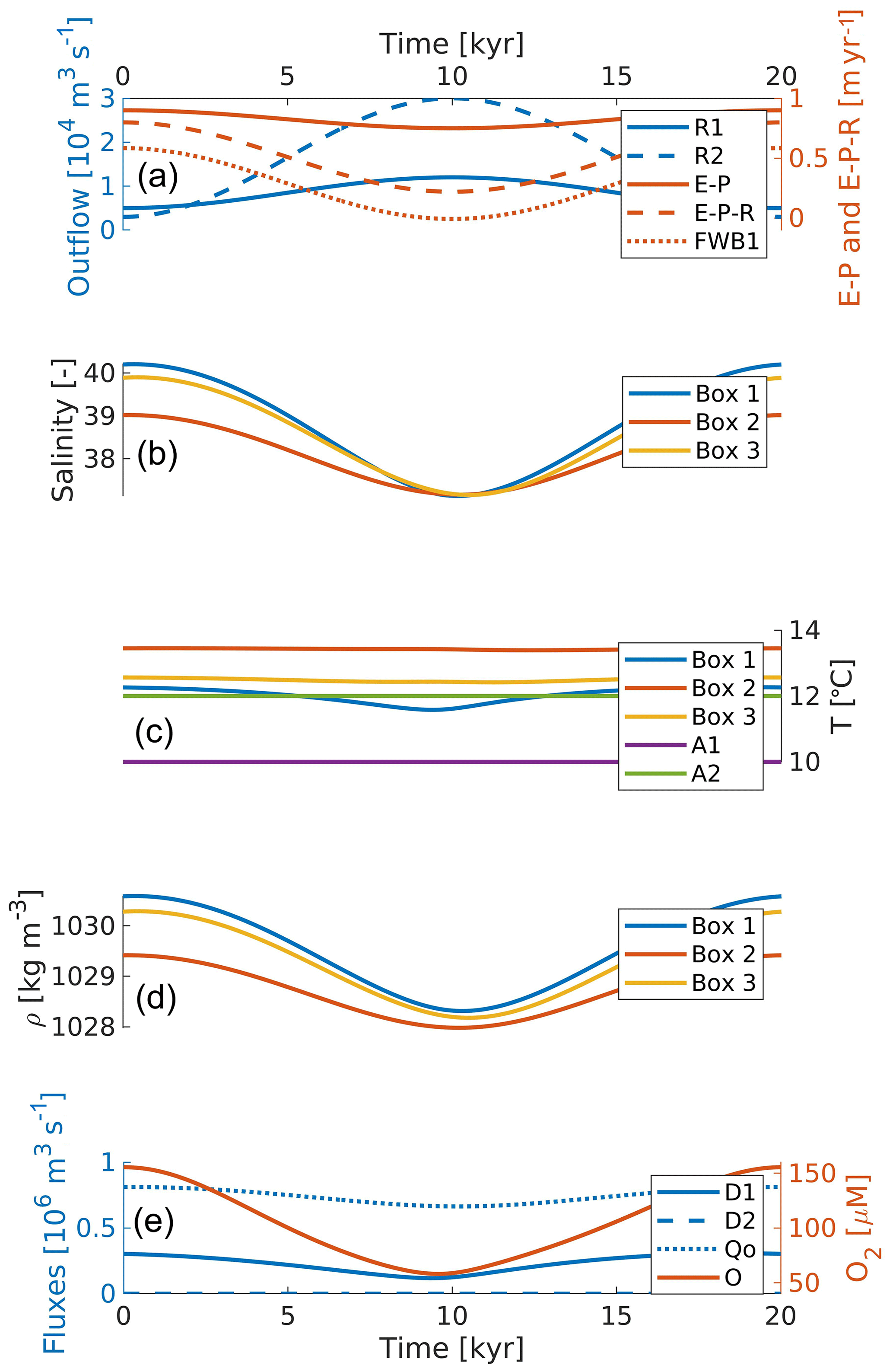
Figure 3The forcing and results of the reference run. (a) The model forcing, with the river outflow on the left axis and the E–P, E–P–R and freshwater budget of box 1 on the right axis. (b–d) The salinity, temperatures and densities for each box, respectively. (e) The relevant fluxes (left axis) and the deepwater oxygen concentration (right axis).
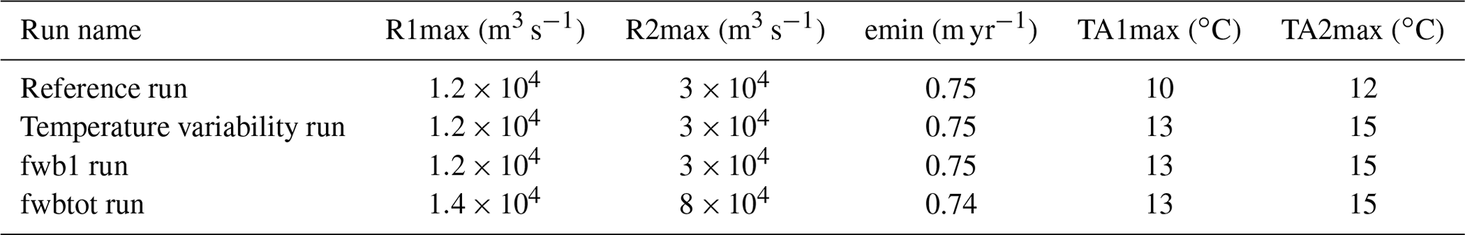
Nile outflow (R2) increases from 5×10³ to 3×10⁴ m3 s−1, while river outflow from Europe only increases from 5×10³ to 1.2×10⁴ m3 s−1 and evaporation decreases from 0.9 to 0.75 m yr−1. While quantitative reconstructions of fluvial discharge and evaporation during sapropel formation are not available, these minimum and maximum values are in agreement with Marzocchi et al. (2015). All other parameters found in Table 1 do not vary with time. Table 2 shows the forcing parameters that are the same for all presented runs, and Table 3 gives the forcing parameters that are changed between runs. As explained in the Introduction we choose these particular runs because they illustrate the sensitivity of the model to the various controlling factors well.
From time 0 towards the precession minimum, the river outflow increases, and as a result salinities decrease, as shown in Fig. 3b. After the precession minimum river outflow decreases again and salinities increase. The differences in salinity between the boxes decrease towards the precession minimum and increase again after the precession minimum. The amplitude of the salinity variability is much smaller in the open Mediterranean box (box 2), as it is connected to the Atlantic (box 0), which has a constant salinity in this run. Deepwater salinity (box 3) lags the salinity of the upper boxes (this will be interpreted after describing the other graphs). As a result of this behaviour, the salinity of the marginal box (box 1) briefly drops below the deepwater salinity just prior to the precession minimum.
The temperatures shown in Fig. 3c do not change drastically, except for a decrease in temperature at the margins in the interval surrounding the precession minimum (we will come back to this below).
As temperature does not change much, density variability (Fig. 3d) is largely determined by changes in salinity. The dip in marginal temperature has an opposite effect on density compared to the salinity fluctuation; consequently, the decrease in the surface-to-deep density gradient is relatively small, and the marginal density does not drop below the deepwater density.
Nevertheless, the decrease in the vertical density difference causes a decrease in DWF (D1 Fig. 3e; see also Eq. 2). DWF in the open Mediterranean box (D2) does not occur in this run, since the density in the upper-open Mediterranean box never exceeds the density of the deepwater box. The cause of the previously mentioned dip in marginal temperature lies in the reduction of DWF, which in turn decreases the inflow of water from the open Mediterranean to the margins (Eq. 12). The decrease in the supply of relatively warm water to the margins causes the water temperature of the margins to approach the much lower atmospheric temperature.
The outflow to the Atlantic (Qo, in Fig. 3d) depends on the density difference between the open Mediterranean and the Atlantic. Since the properties of the Atlantic water are kept constant in all presented model runs, the outflow only depends on the density of the open Mediterranean box. As expected, the decrease in the density of the open Mediterranean water in the interval surrounding the precession minimum causes a slight decrease in outflow to the Atlantic.
The deepwater oxygen concentration (Fig. 3d) depends on (i) oxygen consumption as well as (ii) DWF and vertical mixing. The deepwater oxygen concentration largely follows the same trend as DWF. For roughly 9–20 kyr the deepwater oxygen has a phase lead relative to DWF. Note that DWF does not have to stop completely to cause a decrease in the oxygen concentration; when the oxygen consumption combined with the outflowing oxygen exceeds the supply of new oxygen, the deepwater oxygen concentration decreases.
As we have seen in the description of Fig. 3d, the salinity decrease occurs in both the margins (where the deep water forms in this run) and the open Mediterranean (where the water that flows to the margins originates from). The deepwater salinity depends on DWF and mixing with the overlying boxes. Consequently, the deepwater salinity always lags the salinity of the upper boxes. The amount of lag between the deep and surface boxes depends on the water and property exchange with the deep box and is therefore not constant throughout the run. At the precession minimum, the lag is of the order of 200 years. As the increase in river outflow towards the precession minimum reduces DWF and mixing, the lag between deep and surface–intermediate water salinity also increases (too subtle to see in the graphs). As a result, there is a brief period, starting 1800 years before the precession minimum and ending 440 years after the precession minimum for the margins and 580 years for the open Mediterranean, during which deepwater salinity is higher than surface–intermediate water salinity. Because the changes in density largely depend on salinity in this run and the dip in marginal temperature also slightly leads the precession minimum, it follows that the midpoint of this time interval of minimal DWF falls prior to the precession minimum. The DWF does not stop completely in this run (see Fig. 3e) because the relatively warm open Mediterranean surface–intermediate water keeps the deep water warmer (through mixing) than the marginal water; see Fig. 3. This reference run highlights why the sapropel state is inherently transient: the DWF is only slowed down when the density of the upper boxes is decreasing and increases again when the density starts to return to precession maximum conditions. Since density cannot decrease indefinitely, a state with minimum circulation cannot be maintained.
The deepwater flux at the precession maximum (3×10⁵ m3 s−1) is somewhat lower than found in observational data (1.6×10⁶ m3 s−1; Pinardi et al., 2015), although it is comparable to the DWF of one of the eastern sub-basins (Pinardi et al., 2015). Deepwater oxygen at the precession maximum matches observational data (155 µM in the model versus between 151 and 205 µM observed in the western Mediterranean Sea and 160 to 219 µM in the eastern Mediterranean Sea; Powley et al., 2016). Other conditions, such as temperature and salinity, closely match present-day winter conditions (as reported in Hayes et al., 2019). DWF only occurs at the margins (box 1) in this run; the other deepwater flux is only plotted for easy comparison to other runs (in which it does occur). None of the fluxes change direction in this run, resulting in relatively simple, although not entirely linear, behaviour: the phase relation between the salinities of the boxes is not constant and the temperature of the marginal box, as well as the deepwater oxygen curve, is clearly not sinusoidal. We consider the period with minimal deepwater oxygen concentration, 60 µM, to be the model equivalent of sapropel conditions. Although we only find a very short sapropel (8.8–10.3 kyr) this run demonstrates that the model (i) is capable of approximating the present-day water properties and circulation when forced by present atmospheric conditions and (ii) captures the reduction in DWF expected upon a change to wetter conditions.
3.2 Addition of atmospheric temperature variability
As described in the Introduction, temperature variation due to precession likely also affected buoyancy loss. In order to examine this aspect, we run the model with a 3 ∘C temperature increase at the precession minimum relative to the precession maximum. For atmospheric box A1 the temperature increases from 12 to 15 ∘C, and for box A1 the temperature increases from 10 to 13 ∘C. Both air temperature curves are described by sine waves, as shown in Fig. 4c. We decide to maintain a constant temperature difference between the two atmospheric boxes as there is insufficient evidence for other options. All other parameters are set as described in the reference run.
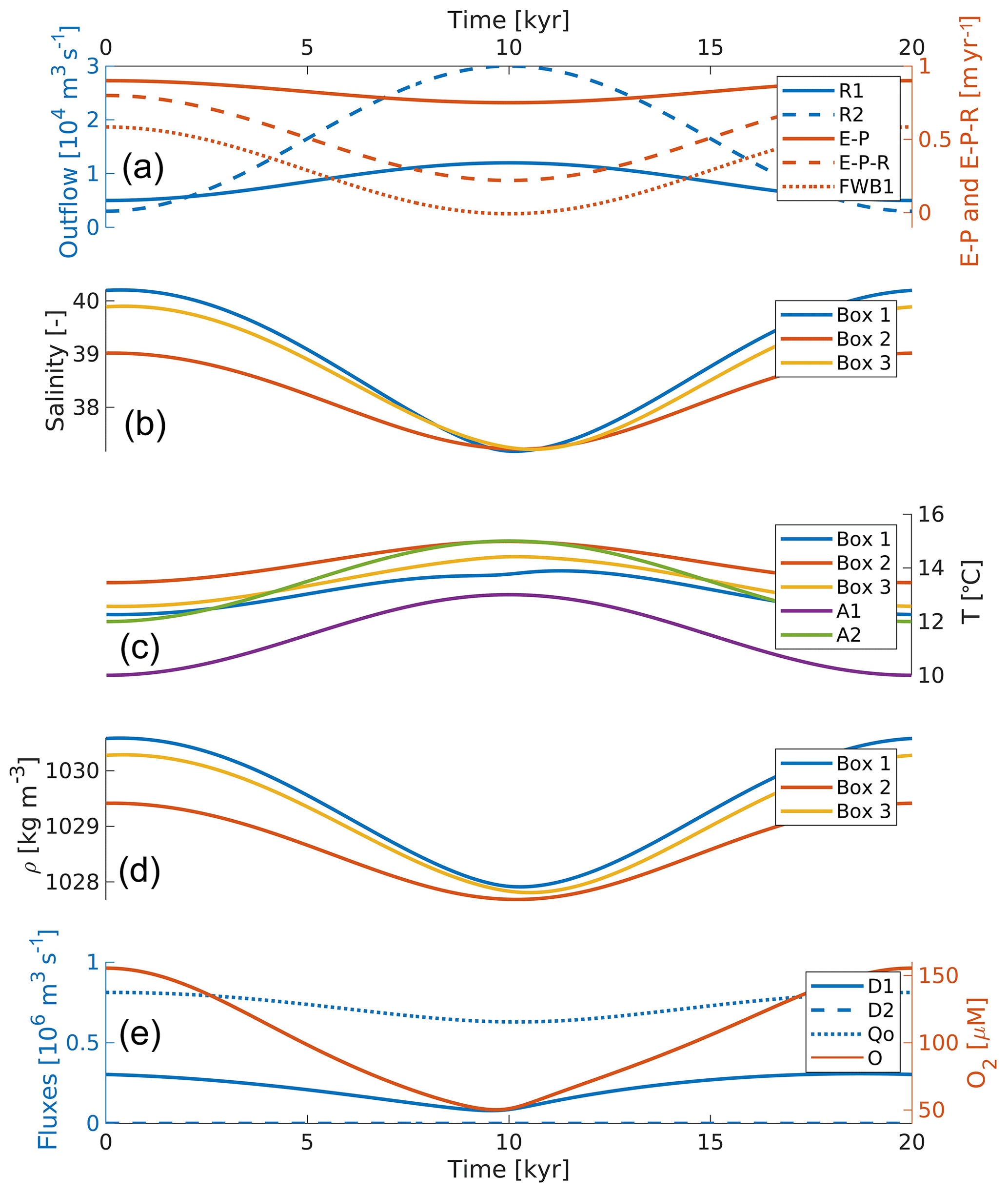
Figure 4The forcing and results of the temperature variability run. The layout of the panels is the same as in Fig. 3.
The overall behaviour of the model is similar to that in the reference run, except that the temperatures of all boxes are now higher during the interval surrounding the precession minimum (Fig. 4c). We still observe a minor decrease in marginal water temperatures at the precession minimum (see Fig. 3c), although it is much smaller than in the reference run since it is now imposed on top of the trend caused by the changing atmospheric temperature. The net effect of a homogeneous basin-wide temperature increase during the precession minimum is a further decrease in DWF during this time interval. We find a sapropel from t=8084 to 10 970 years, which therefore lasts 2013 years, and the midpoint leads the precession minimum by 473 years (see Fig. 4e).
When testing the parameter space, we find that changes in marginal and open Mediterranean air temperature have an opposite effect on DWF: when the air over the margins becomes warmer, heat exchange with the marginal water directly increases the buoyancy of the water involved in DWF, slowing the circulation down. An increase in open Mediterranean air temperature, in contrast, primarily affects the open Mediterranean surface–intermediate water, which mixes with the deep water over a large area. The resulting rise in the temperature of the deep water lowers its density and thereby increases the marginal-to-deepwater density gradient. Since this gradient controls DWF at the margin, an increase in open Mediterranean air temperature ultimately causes an increase in DWF. Since part of the open Mediterranean surface–intermediate water flows to, and mixes with, the marginal water, the effect of the open Mediterranean air temperature increase on the margin–deepwater density gradient is relatively small. This run shows that an atmospheric temperature increase during the precession minimum significantly affects the duration of sapropel conditions in the model. Since both observational and modelling studies find this temperature variability (Marzocchi et al., 2015; Herbert et al., 2015), it will be included in all following model runs.
3.3 Nonlinear behaviour
Next, we explore the effect of a transition to and from a time interval with a positive freshwater budget. Whether or not the freshwater budget of the Mediterranean Sea becomes positive during sapropel formation has been widely debated (Rohling, 1994, and references therein). Although our model cannot directly prove whether or not this has happened, it does allow us to study what the implications for the water properties and circulation would be, which should help in recognizing the expression of a budget switch in the geological record. First we consider a scenario in which only the freshwater budget of the margins becomes positive; in a subsequent run we force the model in such a way that the freshwater budget of the entire basin changes sign.
To have the freshwater budget of the margins become positive, the maximum of R1 is increased from 1.2×10³ to 1.4×10⁴ m3 s−1 (Fig. 5a), and all other parameters are kept the same as in the temperature variability run (Fig. 4), as shown in Table 3 in the row titled “fwb1 run”.
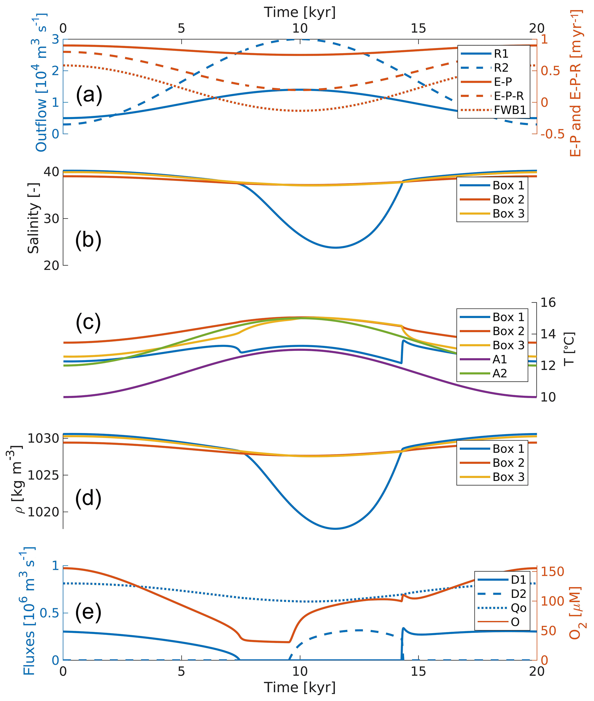
Figure 5The forcing and results of the run in which the freshwater budget of the margins becomes positive for a brief period. The layout of the panels is the same as in Fig. 3.
At a similar timing as the dip in temperature observed in the reference run, we now see a very large decrease in salinity at the margins from 9 to 13 kyr (see Fig. 5b). During this interval we observe that temperatures at the margins approach the temperature of the overlying atmospheric box, while deepwater temperatures approach those found in the open Mediterranean (see Fig. 5c). All are an expression of the disappearance of DWF at the margin (see Fig. 5e; elaborated below), which effectively stops the exchange of the margins with the rest of the basin. Conditions at the margins are mainly determined by river input (causing low salinity) and atmospheric temperature. The properties of the deep water are now only determined by mixing with the open Mediterranean surface–intermediate box and DWF in the same box, explaining the similar temperatures. When the salinity at the margins reaches present-day values again at 13 kyr, we observe a sudden subtle increase in deepwater salinity due to the abrupt increase in DWF at the margin at this moment (see Fig. 5d).
Because the change in salinity is much larger than the change in temperature, the densities of each of the boxes (Fig. 5d) behave similarly as the observed salinities seen in Fig. 5b.
DWF at the margins is found to gradually decrease towards the precession minimum, completely stop at around 8 kyr, and abruptly increase to normal circulation again at around 13 kyr. DWF in the open Mediterranean starts close to the precession minimum and ends abruptly when DWF at the margins starts again. Deepwater oxygen largely correlates with the total DWF, although it reaches a minimum before DWF stops completely and begins to increase only shortly after DWF in the open Mediterranean starts. Similar to previous runs, outflow to the Atlantic (Fig. 5e) is slightly lower during the precession minimum because (i) the density difference between the Atlantic and open Mediterranean surface–intermediate box is smaller, and (ii) the freshwater budget is closer to zero.
We thus find that when the freshwater budget in the marginal box temporarily becomes positive, DWF occurs in the open Mediterranean at the end of the low deepwater oxygen interval (conditions associated with sapropel deposition), thereby terminating this interval early (as shown in Fig. 5). Deepwater mixing with the much less dense water at the margins decreases the density of the deep water, thereby causing DWF in the open Mediterranean box. The result of this is a phase lead of the sapropel midpoint (as a result of the earlier termination) instead of the phase lag commonly reported in the literature (Grant et al., 2016).
In the next run we force the model in such a way that the freshwater budget of the entire basin becomes positive during the interval straddling the precession minimum.
The maximum of R2 is set to 8×10⁴ m3 s−1 and the minimum evaporation to 0.74 m yr−1 (Fig. 6a); all other parameters are kept the same as in the temperature variability run. In the interval from approximately 9 to 13 kyr, the freshwater budget of the entire basin reverses. The changed forcing parameters are shown in Table 3 in the row titled “fwbtot run”.
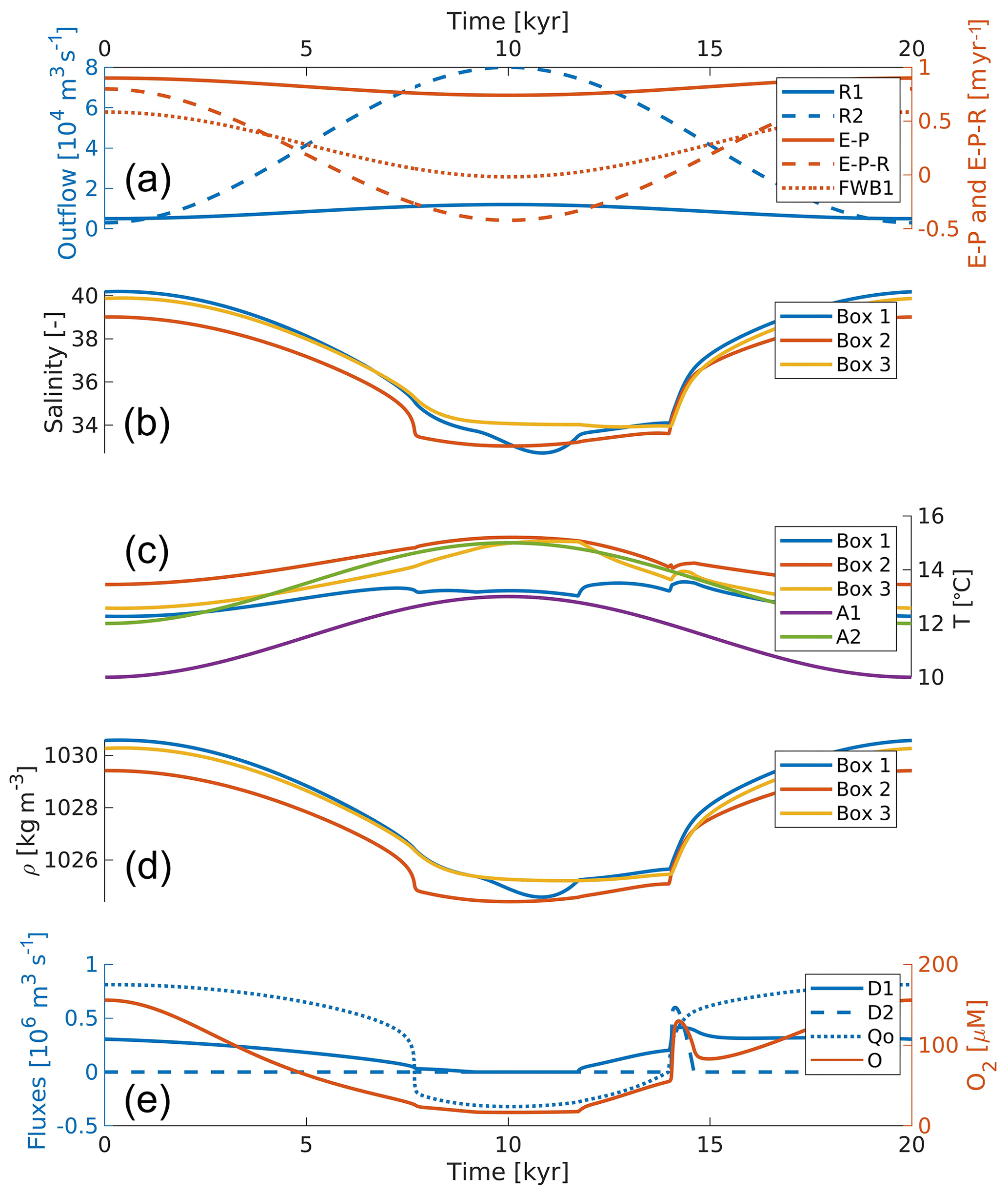
Figure 6The forcing and results of the run in which the freshwater budget of the whole basin becomes positive for a brief period. The layout of the panels is the same as in Fig. 3.
Salinities (Fig. 6b) decrease in response to the decrease in net evaporation. When the freshwater budget reverses, the exchange with the Atlantic decreases, causing less relatively saline water to flow into the upper boxes. Consequently, the salinity of the upper boxes further decreases. The deepwater salinity only begins to decrease more when DWF at the margin starts again. When the freshwater budget becomes negative again, the salinities abruptly increase and then follow the freshwater budget more or less linearly.
The main features of the temperature curves (Fig. 6c) are caused by the same events that are described above for the salinity variability, although temperature is also affected by heat loss to the atmosphere. Consequently, the same main features can be identified, with the difference that (1) the temperature of the upper boxes follows the air temperature curves, and (2) the amplitude is smaller because the heat exchange with the atmosphere acts as negative feedback.
The changes in densities are predominantly determined by salinity, as the changes in temperature are relatively small in this run.
Reversing the freshwater budget also causes the density difference between the Atlantic and open Mediterranean surface–intermediate box to change sign. Consequently, the density-driven flow goes from the Atlantic to the Mediterranean instead of the other way around. In Fig. 6e this is represented by the flux becoming negative. Note that this shift occurs almost instantaneously.
In this run we find a very sharp termination of the sapropel, followed by a brief period with a lower oxygen concentration (as shown in Fig. 6). This is caused by a peak in DWF in both the margin and open Mediterranean when the freshwater budget changes sign. Just prior to the reversal of the freshwater budget, the density of the open Mediterranean surface–intermediate water is much lower than that of the Atlantic water. The reversal of the freshwater budget then causes a rapid increase in surface–intermediate water throughout the basin, resulting in the peak in DWF. The irregularities observed in all runs (such as the occurrence of multiple local minima) in which the freshwater budget of (part of) the basin reverses all strongly depend on the model set-up.
3.4 Phase of evaporation
Recent modelling studies (Marzocchi, 2016) have shown that while evaporation and river outflow are both forced by precession, they may have a different phase relation to their forcing. Runoff and evaporation are the only transient forcings in the presented model runs; therefore, shifting runoff, for example, 2 kyr forward in time gives the exact same wave shape as shifting evaporation 2 kyr backwards in time. The only difference would be that the waveform would be shifted by 4 kyr. Since we are primarily interested in the transient response rather than the absolute timing, we only investigate the effect of the phase of evaporation. To assess the effect of the phase of evaporation on sapropel formation, we calculate the sapropel midpoint and duration for a set of runs with varying evaporation phase (all other parameters remaining unaltered between runs). Apart from the phase of the evaporation forcing, the model is forced exactly the same as in the atmospheric temperature variability experiment (as described in Sect. 3.2).
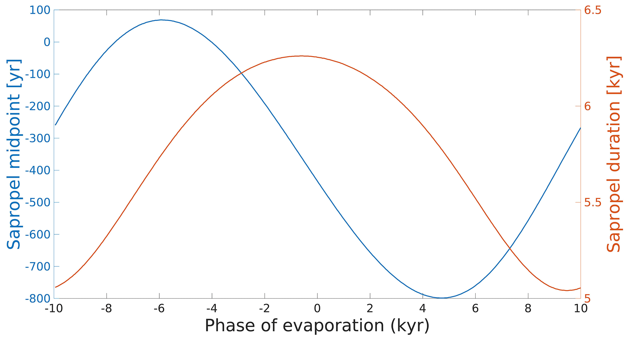
Figure 7Sapropel duration (right axis) and the timing of the midpoint relative to the precession minimum (on the left axis) as a function of the phase of evaporation. Apart from the phase of evaporation, the model forcing is the same as the run in Sect. 3.2.
As shown in Fig. 7, we find a maximum in sapropel duration when evaporation is almost in phase with precession. This is to be expected, as minimum evaporation then coincides with maximum river outflow. Similarly, a minimum in sapropel duration is found when evaporation is almost exactly in anti-phase with precession. Between these peaks the sapropel duration as a function of the phase of evaporation is described by a cosine. The sapropel midpoint is found to vary significantly (up to thousands of years with a large amplitude of evaporation variability) when varying the phase of the evaporation forcing. The shift in sapropel midpoint relative to the precession minimum is at a maximum when evaporation lags or leads approximately 5 kyr. This makes sense, as the minimum in midpoint shift occurs when evaporation is either in phase with precession or in anti-phase (i.e. a shift of 0 or 10 kyr), and the 5 kyr lead or lag falls right between these points. The timing of the midpoint as a function of the phase of evaporation between these extremes is described by a nearly perfect sine wave. Note that the peaks are not exactly at −5 and 5 kyr but slightly shifted; this is likely a result of the equilibrium time of the system.
This experiment, combined with the systematic testing of the parameter space, highlights that although the exact timing and duration depend on the exact forcing, the minimum in deepwater oxygen concentration always occurs close to the precession minimum and the model response is always quasilinear, as long as freshwater budgets are not reversed. We also find that the magnitude of the effect of the phase of evaporation on sapropel timing and duration depends on the amplitude of the evaporation variability (not shown). This makes sense, as the changes in circulation largely respond to freshwater budgets (the only difference between river inflow and evaporation being their respective temperatures) and the amplitude of evaporation variability scales linearly with its impact on the variability of the freshwater budgets.
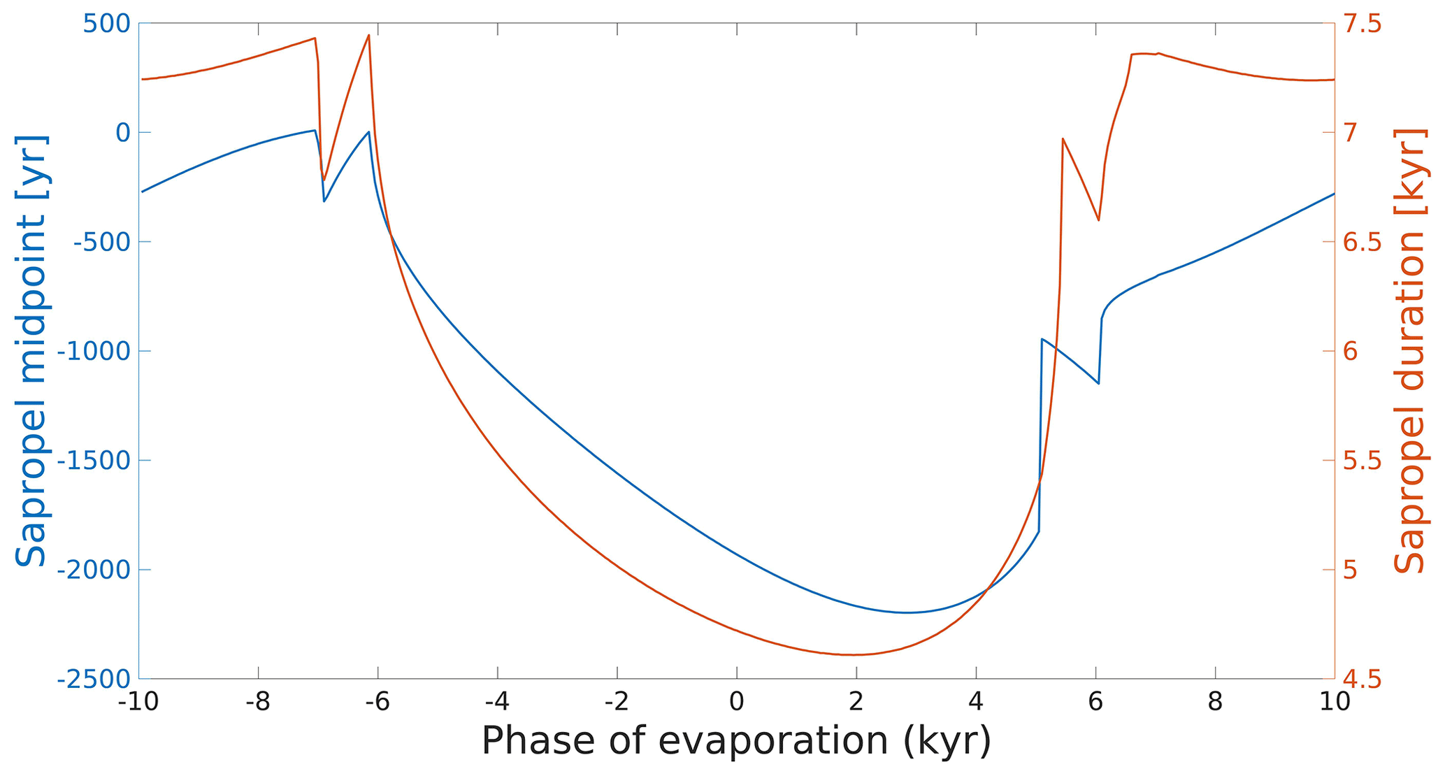
Figure 8Sapropel duration (right axis) and the timing of the midpoint relative to the precession minimum (on the left axis) as a function of the phase of evaporation. Apart from the phase of evaporation, the model forcing is the same as the first run in Sect. 3.3.
When systematically varying the components of the water budget within the limits mentioned in the model set-up, we find that in the regimes in which the freshwater budget of (part of) the basin changes sign, sapropels are cut short considerably. When performing the same analyses described above but using the forcing of the first run in Sect. 3.3, we find that this causes the midpoint of the sapropel to occur prior to the precession minimum (Fig. 8). Note that runs with multiple sapropel intervals cannot be described as having a single midpoint or duration.
4.1 Model convergence
The time step of 1 year naturally results from the concept that deep water forms during winter storms, making it the highest resolution possible as long as seasonal variability is not included. From a purely mathematical perspective, however, the time resolution should not affect the outcome significantly, as long as a sufficiently small time step is used to prevent aliasing. We tested this by varying the temporal resolution given a certain forcing. We find no significantly different results with a time step below 10 years. With a time step larger than 10 years, aliasing occurs. We conclude that a time step of 1 year is sufficient for the analyses in this study.
4.2 The role of assumptions and simplifications
All models require assumptions and simplifications to be made, as they are by design a simplified version of (part of) a system. Simple box models, such as the model presented in this paper, aim to identify the smallest subset of processes that can describe a certain phenomenon. As such, this model represents a generic semi-enclosed basin given that no specific geometry is included. This implies that by altering the parameter values and in some cases the strait exchange equations, the model can easily be adapted to other semi-enclosed basins, such as the Black Sea.
In our model we parameterize intra-annual variability. Including seasonality would require separate intermediate water boxes (increasing complexity), while for the oxygenation of deep water only the amount of DWF and mixing with the overlying water mass is truly relevant. Furthermore, we would have to make assumptions regarding the annual variability of the forcing parameters (river outflow and evaporation), which are not well constrained for geological history. We therefore decided to parameterize the seasonal variability by calculating a yearly averaged DWF flux based on winter temperatures. This allows us to study the fundamental mechanisms of sapropel formation. OGCMs would be more appropriate to study the role of seasonal variation.
We do not include separate boxes for the eastern and western Mediterranean in our model. The aim of a conceptual model is to capture the first-order aspects of a process with a minimal set-up. The current set-up does this. Incorporating separate sub-basins would imply doubling the number of boxes and would also double the number of forcing parameters and equations, all of which adds uncertainty to the model (quantitative reconstructions do not exist for most of these parameters). Moreover, the complexity quickly increases, making it much harder to test and describe the parameter space and identify key mechanisms. While this could be tested in a future study, we find it important to first understand the behaviour of the a semi-enclosed basin with a gateway before studying what is essentially a second-order system. We expect that the effect in the eastern basin is similar to the difference between a first-order and second-order filter: a larger shift of the midpoint (larger group delay) and likely a higher sensitivity in the eastern basin. Any resonances in the system are also expected to become more prominent (since the resonant frequencies are now amplified twice).
The model forcing used in this study is chosen to reflect either the variability envisaged in the commonly accepted mechanism (as sketched in Sect. 1.1) or oceanographic and climatic variability deduced from modelling studies and the geological record as accurately as possible. Other processes such as the North Atlantic oscillation and solar activity are not taken into account because they are not thought to be of first-order importance for sapropel formation, as described in Rossignol-Strick (1985) and Rohling et al. (2015), for example. While these processes likely influence sapropel formation, they are unlikely to be essential.
Besides precession, obliquity also affects sapropel formation, but it is not our aim to reconstruct the exact conditions during specific time intervals. For an individual sapropel, adding an obliquity component would effectively slightly modulate the frequency and amplitude of the forcing. Since the model is not very sensitive to the exact frequency of the forcing and we already extensively tested the parameter space in terms of amplitude, a simple (20 kyr) sine wave suffices as forcing. Also note that since obliquity does not have a harmonic relation with precession, the modulation would not have the same effect on every sapropel. It likely affects the thickness of a sapropel, for example, but the effect may work both ways when comparing different sapropels.
The model output comprises an average value for deepwater oxygen as the deep water is a single box. In reality, however, oxygen concentrations vary spatially. A prime example of this is the absence of sapropels in most of the western Mediterranean Sea. This abstraction should be taken into consideration when interpreting the model results. This model focusses on the transient response of water fluxes in the Mediterranean Sea, and the oxygen output is calculated to get a first-order impression of deepwater ventilation. A biogeochemical model, similar to the one presented in Slomp and Van Cappellen (2007), would have to be included to specifically study bottom-water oxygenation. We expect that the main difference with a biogeochemical model is that in our model river input directly affects oxygen consumption, while the surface–intermediate boxes would act as a reservoir for nutrients (with their own feedbacks) in the biogeochemical model, thereby delaying the response to changes in river input.
Note finally that in reality DWF occurs following two different mechanisms (open-ocean convection and mixing of the water at margins during winter storms, which then cascades to the deep basin; see Sect. 1.1), and in multiple sub-basins that each have their own conditions. The regime in Fig. 5 relies on the freshwater budget of the margins changing sign. In reality there are many different marginal water masses in the sub-basins rather than one single “margin”. This makes it likely that the freshwater budget becoming positive in any one of these sub-basins will have similar consequences for the circulation. Since the freshwater budgets of these basins are independent, it would be possible to drastically alter the circulation multiple times during a single precession cycle. Presently, the Adriatic Sea has a positive freshwater budget (Raicich, 1996), and the Aegean Sea is known to have had a positive freshwater budget in the past (Zervakis et al., 2004).
The simplicity of the model makes it especially suitable for describing transient, nonlinear behaviour, allowing for the identification of crucial mechanisms. More complex models, while providing other benefits, are generally too difficult to interpret on this level or do not allow for runs of sufficient length to study the transient response over a full precession cycle. The presented model runs give an overview of the behaviour of the model. When systematically testing the parameter space, we find that this behaviour largely depends on the general trends and reversal of freshwater budgets rather than specific forcing or parameter choices. This makes the results of the study much more robust and meaningful.
Exchange with the Black Sea also affects circulation in the Mediterranean Sea (Soulet et al., 2013, show increased runoff during HS1). For sapropels during which there is exchange through the Bosphorus Strait, the exchange is not constant through time and also depends on the inflow of Mediterranean water into the Black Sea. Opening or closing the strait prior to or during a sapropel may impact the circulation. When the sill becomes deep enough to allow for a two-layer exchange, a large amount of saline water would flow into the Black Sea (following the same principle as at the Strait of Gibraltar), thereby causing extra, relatively fresh water to flow out into the Mediterranean Sea. During some sapropels, the strait may have been closed. Furthermore, there are very few data regarding the exchange of opening and closing the Bosphorus Strait prior to the most recent opening (approximately 11 ka), perhaps with the exception of the Pontian (which is beyond the scope of this paper). Consequently, we do not include exchange with the Black Sea. For the cases in which there was a steady outflow of fresh water (or an exchange that can be parameterized as such) this could indeed be seen as an extra freshwater source for the margins. We have already tested this effect by varying the river outflow into the margins.
Meltwater pulses likely affect sapropel formation, but we do not consider them to be of first-order importance. During many sapropels, meltwater pulses did not occur. In future applications of this model for which a specific sapropel and/or interval is studied, drivers such as meltwater pulses should be included.
4.3 Describing nonlinear relationships and transient response
The occurrence of sapropels is often considered from a binary perspective: a sediment is either a sapropel, or it is not. The dominant forcing mechanism (astronomic variability), however, can be easily described by a combination of a limited number of sine waves: the resonant frequencies of the planetary bodies in our solar system (for example, Laskar, 1988). For a single sapropel, only climatic precession – a nearly a perfect sine – is considered to be of first-order importance in controlling bottom-water oxygenation (Rossignol-Strick, 1985), with the rest of the orbital configuration mostly modulating the effect of precession. If a model strives to capture the current hypothesis of sapropel formation starting from astronomic variability, it must therefore transform a sine wave into something that is not a sine wave, requiring the model to be nonlinear. Our model allows for such behaviour. Even when considering intra-sapropel variability, thereby surpassing a binary approach, the sapropel record is clearly not sinusoidal (see, for example, Grant et al., 2016; Dirksen et al., 2019).
One of the main research questions of this study is when sapropel formation occurs. In a linear system, one would simply calculate the phase of the output with respect to the input. However, as the output is no longer linearly related to the input, this is not possible. A simple threshold analysis is not ideal either, as the cut-off level can have a major impact on both timing and duration, while a clear definition is not readily available. Furthermore, even when the threshold is defined, this method would not be usable for sapropelic marls, which are thought to be the result of the same process but do not share the same chemical composition. We partly avoid this problem by not only considering the midpoint of the sapropel (when assuming a certain oxygen threshold; see Sect. 4.5), but also the full waveform (e.g. which intervals could be sapropelic with a slightly different forcing). In the sedimentary record this is generally not possible, since the non-sapropelic intervals do not record all parameters and are often bioturbated. So while our approach cannot be applied to the sedimentary record, it does give insight into the factors that influence sapropel timing. Even this definition of sapropel timing becomes problematic when one or more interruptions occur, since in that case there is more than one midpoint.
We find that, when using realistic model forcing, stable sapropel conditions do not occur. Even when using constant forcing, a permanent complete stop of DWF either does not occur or only occurs under very specific conditions. Note that in the Black Sea permanent stratification does appear to occur, but here, the positive freshwater budget allows some of the water flowing into the Black Sea at the Bosphorus Strait to sink to the deep water (Bogdanova, 1963), keeping it relatively saline and dense. However, our results indicate that sapropel conditions can occur transiently without a positive freshwater budget, with realistic forcing. We therefore conclude that studying the oceanographic state during sapropel conditions by modelling steady-state conditions with a stratified water column results in a very limited understanding of sapropel formation.
4.4 Comparison with geological data and other models
Comparing model results to geological data is most effective when an accurate age model is available for the geological data. We therefore only consider the five youngest sapropels in this paper. The most recent sapropel (S1) is thought to have been triggered by sea level rise, which in turn resulted in a connection between the Black Sea and the Mediterranean Sea (Rohling et al., 2015). As both sea level variability and exchange through the Bosphorus Strait are beyond the scope of this paper, sapropel S1 is not suitable for comparison. We therefore focus on sapropels S3, S4 and S5 in the rest of the section.
In the run with variable air temperature (Fig. 4), the modelled sapropel duration and timing are within the dating uncertainty of what has been found for sapropel S3 and S4 in core LC21 (Grant et al., 2016). Note that the same study finds that sapropels S1 and S5 lag precession by 2.1–3.3 kyr. This suggests that our model is capable of capturing the most relevant mechanisms for S3 and S4 but that other features not included in the model affected the timing of S1 and S5. For S5 there is evidence suggesting that the Black Sea reconnected to the Mediterranean Sea within the dating uncertainty of the onset of sapropel S5 (Grant et al., 2016, 2012; Wegwerth et al., 2014)
It should be noted that while the model often shows a midpoint lag (relative to the insolation minimum) of a few hundred years, uncertainties related to radiometric dating methods are often larger. However, we find that midpoint lag becomes larger with decreasing strait efficiency, implying that during times with low sea level or otherwise restricted exchange, the lag might become very relevant. A prime example of such a case would be the Messinian salinity crisis and the surrounding intervals (Topper and Meijer, 2015). Moreover, as shown in Figs. 5 and 6, alternative regimes (in which the freshwater budget of either part of the basin or the entire basin changes sign) can shift the midpoint of the sapropel considerably, as shown in Fig. 8. Unlike the relatively minor shifts in midpoint resulting from only changing the phase of evaporation, the resulting difference in sapropel timing is sufficiently large to be detectable in the geological record.
De Lange et al. (2008) find that the freshening of the surface waters starts earlier and lasts longer than the suboxic bottom-water conditions during S1. Our model also shows this behaviour in all of the presented runs (most notably in Figs. 3, 4 and 6). This makes sense as DWF does not stop completely when the surface water starts to become less saline; it is only reduced slowly. Furthermore, the oxygen has to be depleted for suboxic conditions to occur; this is limited by oxygen consumption and further slowed down by vertical mixing and DWF. How much longer the period of reduced sea surface salinity lasts compared to the period of suboxic bottom water likely depends on the exact location and water depth. The model is therefore mostly useful to gain insight into the mechanisms rather than the exact timing.
The regime described in Fig. 6 can show a sudden termination of the sapropel, which is similar to that seen in records of sapropel S5 (Dirksen et al., 2019). In the model such a sudden termination can only be achieved through DWF in the open Mediterranean by reversing the freshwater budget of the entire Mediterranean. The coupling between the margins and deep water is insufficient to cause such a sudden termination. This suggests that during S5 the freshwater budget of part of the basin or the whole basin potentially reversed. Such a large change in the freshwater budget is in line with Bale et al. (2019), who found that surface salinities in three different cores in the eastern Mediterranean were sufficiently low to support free-living heterocystous cyanobacteria during sapropel S5. Moreover, oceanographic conditions may differ significantly between different parts of the basin: the oxygen concentration (and related variables) of a hypothetical core taken at the margin would be expected to show a pattern more similar to the DWF in the marginal box, while a core in the open Mediterranean may be more similar to the open Mediterranean surface–intermediate water box.
Sapropel interruptions commonly occur in the stratigraphic record (for example, in S5 in core LC21; Rohling et al., 2006, 2015). With slightly different settings, the sharp peak in deepwater oxygen in Fig. 6e can be made to occur earlier and less intensely, resulting in an interrupted sapropel. The model therefore suggests that such interruptions can occur without further external forcing. This hypothesis could be tested in the stratigraphic record by looking for evidence of a reversed freshwater budget of (part of) the basin during such interrupted sapropels and constructing high-resolution intra-sapropel age models to assess the relative timing of the relevant features compared to insolation.
Each sapropel in the geological record is different; this becomes apparent when considering the most recent six: S1 has a different timing and is likely related to sea level variability (Grant et al., 2016; Hennekam, 2015; Grimm et al., 2015). S2 is not found at all. S4 has interruptions in core LC21 (Grant et al., 2012), and high-resolution records of, for example, trace metals show very different characteristics. In the same core, the timing of the midpoint of S3 and S4 compared to insolation is the same, while that of S1 and S5 is different. S5 is much longer than all of the previous sapropels, does not have any burn down at least one location (Dirksen et al., 2019), has an interruption in other locations (Rohling et al., 2006) and again shows generally different characteristics in different cores (Dirksen et al., 2019; Grant et al., 2016; Rohling et al., 2006). S6 again looks very different.
We conclude that both in the geological record and in the model, a typical sapropel does not exist. The timing and mechanisms involved may differ considerably between sapropels and locations, as highlighted by our model results. Moreover, we find that an increase in freshwater budget alone is not sufficient to describe all key aspects of sapropel formation. An increase in atmospheric temperatures during the precession minimum (as observed in data and modelling studies; Marzocchi et al., 2015; Herbert et al., 2015) directly affects buoyancy loss during the interval in which sapropels form. This makes atmospheric temperature variability an integral feature of the system. Without it unrealistic evaporation or river outflow is needed to result in sufficiently long sapropels. Our model results support this hypothesis.
The analysis presented in this paper illustrates that relatively simple models can give new, fundamental insights into the physical processes driving sapropel formation. The timing of sapropels relative to insolation has been widely studied in the sedimentary record. On the basis of our novel long-duration experiments we find that the timing of sapropels is very sensitive to the exact climatologic and oceanographic conditions. The nonlinear response to insolation forcing implies that the sapropel record does not have a linear phase relation with insolation. The strongly nonlinear regimes in our model highlight that the midpoint of a sapropel (the average of the ages of the top and bottom of the sapropel) can be shifted significantly with a minor change in forcing by cutting it short with a sudden termination, while during the rest of the precession cycle the response can be very similar to the nearly linear regime presented in the reference experiment. Our model results suggest that an increase in freshwater input alone, as in the general hypothesis for sapropel formation, does not provide a sufficient reduction in buoyancy loss to form sapropels as they are found in the geological record. We propose that precession-controlled atmospheric temperature variability also plays a key role in the process of sapropel formation.
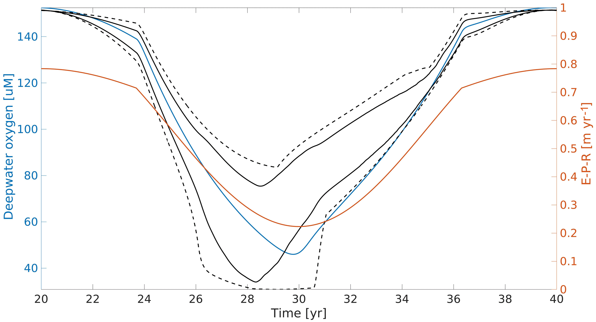
Figure A1An example of the sensitivity analyses. Here the maximum of R1 is varied randomly by up to 5×10³ m3 s−1 above or below the general setting over 200 runs. The blue line indicates the initial run, the solid black lines indicate the upper and lower 1σ of each point in time, and the black dashed lines indicate the minimum and maximum.
No data sets were used in this article.
PM conceived the basic idea. JPD elaborated the concepts and performed the analyses. Both authors contributed to the model set-up and the writing of the paper.
The authors declare that they have no conflict of interest.
The authors would like to thank Ronja Ebner for the many useful discussions and her help with checking the formulas. We thank the editor (Alberto Reyes) and three anonymous reviewers for their thoughtful and constructive comments.
This research has been supported by the Netherlands Research Centre for Integrated Solid Earth Science (grant no. ISES 2017-UU-23).
This paper was edited by Alberto Reyes and reviewed by three anonymous referees.
Adloff, F., Mikolajewicz, U., Kučera, M., Grimm, R., Maier-Reimer, E., Schmiedl, G., and Emeis, K.-C.: Upper ocean climate of the Eastern Mediterranean Sea during the Holocene Insolation Maximum – a model study, Clim. Past, 7, 1103–1122, https://doi.org/10.5194/cp-7-1103-2011, 2011. a
Amies, J., Rohling, E. J., and Grant, K. M.: Quantification of African Monsoon Runoff During Last Interglacial Sapropel S5, Paleoceanogr. Paleocl., 34, 1–30, https://doi.org/10.1029/2019PA003652, 2019. a, b, c, d
Ashkenazy, Y., Stone, P. H., and Malanotte-Rizzoli, P.: Box modeling of the Eastern Mediterranean sea, Physica A, 391, 1519–1531, https://doi.org/10.1016/j.physa.2011.08.026, 2012. a
Bale, N. J., Hennekam, R., Hopmans, E. C., Dorhout, D., Reichart, G.-j., Meer, M. V. D., Villareal, T. A., Damsté, J. S. S., and Schouten, S.: Biomarker evidence for nitrogen-fixing cyanobacterial blooms in a brackish surface layer in the Nile River plume during sapropel deposition, Geology, XX, 1–5, https://doi.org/10.1130/G46682.1, 2019. a
Bensi, M., Cardin, V., Rubino, A., Notarstefano, G., and Poulain, P. M.: Effects of winter convection on the deep layer of the Southern Adriatic Sea in 2012, J. Geophys. Res.-Oceans, 118, 6064–6075, https://doi.org/10.1002/2013JC009432, 2013. a
Bianchi, D., Zavatarelli, M., Pinardi, N., Capozzi, R., Capotondi, L., Corselli, C., and Masina, S.: Simulations of ecosystem response during the sapropel S1 deposition event, Palaeogeogr. Palaeocl., 235, 265–287, https://doi.org/10.1016/j.palaeo.2005.09.032, 2006. a, b, c
Bigg, G. R.: An ocean general circulation model view of the glacial Mediterranean thermohaline circulation, Paleoceanography, 9, 705–722, https://doi.org/10.1029/94PA01183, 1994. a, b
Bogdanova, A. K.: The distribution of Mediterranean waters in the Black Sea, Deep-Sea Res., 10, 665–672, https://doi.org/10.1016/0011-7471(63)90014-7, 1963. a
Bryden, H. L. and Kinder, T. H.: Steady two-layer exchange through the Strait of Gibraltar, Deep-Sea Res. Pt. I, 38, S445–S463, https://doi.org/10.1016/s0198-0149(12)80020-3, 1991. a
Calvert, S. E., Nielsen, B., and Fontugne, M. R.: Evidence from nitrogen isotope ratios for enhanced productivity during formation of eastern Mediterranean sapropels, Nature, 359, 223–225, https://doi.org/10.1038/359223a0, 1992. a
Channell, J. E. T., Hodell, D. A., Singer, B. S., and Xuan, C.: Reconciling astrochronological and 40Ar∕39Ar ages for the Matuyama-Brunhes boundary and late Matuyama Chron, Geochem. Geophy. Geosy., 11, 12, https://doi.org/10.1029/2010gc003203, 2010. a
Command, N. O.: US Navy climatic study of the Mediterranean Sea, Naval Oceanography Command Detachment, Asheville, North Carolina, 342 pp., 1987. a
Cramp, A. and O'Sullivan, G.: Neogene sapropels in the Mediterranean: A review, Mar. Geol., 153, 11–28, https://doi.org/10.1016/S0025-3227(98)00092-9, 1999. a
De Lange, G. and Ten Haven, H.: Recent sapropel formation in the eastern Mediterranean, Nature, 305, 797–798, https://doi.org/10.1038/305797a0, 1983. a
De Lange, G. J., Thomson, J., Reitz, A., Slomp, C. P., Speranza Principato, M., Erba, E., and Corselli, C.: Synchronous basin-wide formation and redox-controlled preservation of a Mediterranean sapropel, Nat. Geosci., 1, 606–610, https://doi.org/10.1038/ngeo283, 2008. a, b
Dirksen, J. P., Hennekam, R., Geerken, E., and Reichart, G. J.: A Novel Approach Using Time-Depth Distortions to Assess Multicentennial Variability in Deep-Sea Oxygen Deficiency in the Eastern Mediterranean Sea During Sapropel S5, Paleoceanogr. Paleocl., 34, 774–786, https://doi.org/10.1029/2018PA003458, 2019. a, b, c, d
Finnigan, T. D., Winters, K. B., and Ivey, G. N.: Response Characteristics of a Buoyancy-Driven Sea, J. Phys. Oceanogr., 31, 2721–2736, https://doi.org/10.1175/1520-0485(2001)031<2721:RCOABD>2.0.CO;2, 2001. a
Gertmann, I., Ovchinnikov, I., and Popv, Y.: Deep convection in the eastern basin of the Mediterranean Sea, Oceanology, 34, 19–25, 1994. a
Gertman, I., Pinardi, N., Popov, Y., and Hecht, A.: Aegean sea water masses during the early stages of the Eastern Mediterranean Climatic Transient (1988–90), J. Phys. Oceanogr., 36, 1841–1859, https://doi.org/10.1175/JPO2940.1, 2006. a
Grant, K. M., Rohling, E. J., Bar-Matthews, M., Ayalon, A., Medina-Elizalde, M., Ramsey, C. B., Satow, C., and Roberts, A. P.: Rapid coupling between ice volume and polar temperature over the past 50,000 years, Nature, 491, 744–747, https://doi.org/10.1038/nature11593, 2012. a, b
Grant, K. M., Grimm, R., Mikolajewicz, U., Marino, G., Ziegler, M., and Rohling, E. J.: The timing of Mediterranean sapropel deposition relative to insolation, sea-level and African monsoon changes, Quaternary Sci. Rev., 140, 125–141, https://doi.org/10.1016/j.quascirev.2016.03.026, 2016. a, b, c, d, e, f
Grimm, R., Maier-Reimer, E., Mikolajewicz, U., Schmiedl, G., Müller-Navarra, K., Adloff, F., Grant, K. M., Ziegler, M., Lourens, L. J., and Emeis, K. C.: Late glacial initiation of Holocene eastern Mediterranean sapropel formation, Nat. Commun., 6, 1, https://doi.org/10.1038/ncomms8099, 2015. a, b
Hayes, D. R., Schroeder, K., Poulain, P.-M., Testor, P., Mortier, L., Bosse, A., and du Madron, X.: 18 Review of the Circulation and Characteristics of Intermediate Water Masses of the Mediterranean: Implications for Cold-Water Coral Habitats, 9, 195–211, https://doi.org/10.1007/978-3-319-91608-8_18, 2019. a, b, c
Hennekam, R.: High-frequency climate variability in the late Quaternary eastern Mediterranean Associations of Nile discharge and basin overturning circulation dynamics, no. 78 in Utrecht Stud. Earth Sci., UU Dept. of Earth Sciences, 2015. a
Herbert, T. D., Ng, G., and Peterson, L. C.: Evolution of Mediterranean sea surface temperatures 3.5–1.5 Ma: regional and hemispheric influences, Earth Planet. Sc. Lett., 409, 307–318, 2015. a, b, c
Herrmann, M., Estournel, C., Déqué, M., Marsaleix, P., Sevault, F., and Somot, S.: Dense water formation in the Gulf of Lions shelf: Impact of atmospheric interannual variability and climate change, Cont. Shelf Res., 28, 2092–2112, https://doi.org/10.1016/j.csr.2008.03.003, 2008. a
Hilgen, F. J.: Extension of the astronomically calibrated (polarity) time scale to the Miocene/Pliocene boundary, Earth Planet. Sc. Lett., 107, 349–368, https://doi.org/10.1016/0012-821X(91)90082-S, 1991. a
Hilgen, F. J., Krijgsman, W., Langereis, C. G., Lourens, L. J., Santarelli, A., and Zachariasse, W. J.: Extending the astronomical (polarity) time scale into the Miocene, Earth Planet. Sc. Lett., 136, 495–510, https://doi.org/10.1016/0012-821X(95)00207-S, 1995. a
Jordà, G., Von Schuckmann, K., Josey, S. A., Caniaux, G., García-Lafuente, J., Sammartino, S., Özsoy, E., Polcher, J., Notarstefano, G., Poulain, P. M., Adloff, F., Salat, J., Naranjo, C., Schroeder, K., Chiggiato, J., Sannino, G., and Macías, D.: The Mediterranean Sea heat and mass budgets: Estimates, uncertainties and perspectives, Prog. Oceanogr., 156, 174–208, https://doi.org/10.1016/j.pocean.2017.07.001, 2017. a
Kemp, A. E., Pearce, R. B., Koizumi, I., Pike, J., and Rance, S. J.: The role of mat-forming diatoms in the formation of Mediterranean sapropels, Nature, 398, 84–84, https://doi.org/10.1038/20011, 1999. a
Krijgsman, W., Hilgen, F. J., Raffi, I., Sierro, F. J., and Wilson, D. S.: Chronology, causes and progression of the Messinian salinity crisis, Nature, 400, 652–655, https://doi.org/10.1038/23231, 1999. a
Laskar, J.: Secular evolution of the solar system over 10 million years, Astron. Astrophys., 198, 341–362, 1988. a
Lourens, L. J., Antonarakou, A., Hilgen, F. J., Van Hoof, A. A., Vergnaud-Grazzini, C., and Zachariasse, W. J.: Evaluation of the Plio-Pleistocene astronomical timescale, Paleoceanography, 11, 391–413, https://doi.org/10.1029/96PA01125, 1996. a
Malanotte-Rizzoli, P.: The northern adriatic sea as a prototype of convection and water mass formation on the continental shelf, Elsevier Oceanography Series, 57, 229–239, https://doi.org/10.1016/S0422-9894(08)70070-9, 1991. a
Marshall, J. and Schott, F.: Open-ocean convection: Observations, theory, and models, Rev. Geophys., 37, 1–64, https://doi.org/10.1029/98RG02739, 1999. a
Marzocchi, A.: Modelling the impact of orbital forcing on late Miocene climate: implications for the Mediterranean Sea and the Messinian Salinity Crisis, PhD thesis, University of Bristol, 2016. a
Marzocchi, A., Lunt, D. J., Flecker, R., Bradshaw, C. D., Farnsworth, A., and Hilgen, F. J.: Orbital control on late Miocene climate and the North African monsoon: insight from an ensemble of sub-precessional simulations, Clim. Past, 11, 1271–1295, https://doi.org/10.5194/cp-11-1271-2015, 2015. a, b, c, d
Matthiesen, S. and Haines, K.: A hydraulic box model study of the Mediterranean response to postglacial sea-level rise, Paleoceanography, 18, 4, https://doi.org/10.1029/2003PA000880, 2003. a, b, c
Meijer, P. Th. and Dijkstra, H. A.: The response of Mediterranean thermohaline circulation to climate change: a minimal model, Clim. Past, 5, 713–720, https://doi.org/10.5194/cp-5-713-2009, 2009. a, b, c
Meijer, P. T. and Tuenter, E.: The effect of precession-induced changes in the Mediterranean freshwater budget on circulation at shallow and intermediate depth, J. Mar. Syst., 68, 349–365, https://doi.org/10.1016/j.jmarsys.2007.01.006, 2007. a
Mikolajewicz, U.: Modeling Mediterranean Ocean climate of the Last Glacial Maximum, Clim. Past, 7, 161–180, https://doi.org/10.5194/cp-7-161-2011, 2011. a
Myers, P. G.: Flux-forced simulations of the paleocirculation of the Mediterranean, Paleoceanography, 17, 9-1–9-7, https://doi.org/10.1029/2000pa000613, 2002. a
Myers, P. G. and Rohling, E. J.: Modeling a 200-Yr interruption of the Holocene Sapropel S1, Quaternary Res., 53, 98–104, https://doi.org/10.1006/qres.1999.2100, 2000. a
Myers, P. G., Haines, K., and Rohling, E. J.: Modeling the paleocirculation of the Mediterranean: The last glacial maximum and the Holocene with emphasis on the formation of sapropel S1, Paleoceanography, 13, 586–606, https://doi.org/10.1029/98PA02736, 1998. a
Joint Panel on Oceanographic Tables: Progress on oceanographic tables and standards, 1983–1986: work and recommendations of the Unesco/SCOR/ICES/IAPSO Joint Panel, no. 50 in UNESCO Tech. Pap. Mar., Unesco, 1986. a
Pinardi, N., Zavatarelli, M., Adani, M., Coppini, G., Fratianni, C., Oddo, P., Simoncelli, S., Tonani, M., Lyubartsev, V., Dobricic, S., and Bonaduce, A.: Mediterranean Sea large-scale low-frequency ocean variability and water mass formation rates from 1987 to 2007: A retrospective analysis, Prog. Oceanogr., 132, 318–332, https://doi.org/10.1016/j.pocean.2013.11.003, 2015. a, b
Powley, H. R., Krom, M. D., and Van Cappellen, P.: Circulation and oxygen cycling in the Mediterranean Sea: Sensitivity to future climate change, J. Geophys. Res.-Oceans, 121, 8230–8247, 2016. a, b
Raicich, F.: On the fresh water balance of the Adriatic Sea, J. Mar. Syst., 9, 305–319, https://doi.org/10.1016/S0924-7963(96)00042-5, 1996. a
Roether, W., Manca, B. B., Klein, B., Bregant, D., Georgopoulos, D., Beitzel, V., Kovačević, V., and Luchetta, A.: Recent changes in eastern Mediterranean deep waters, Science, 271, 333–335, https://doi.org/10.1126/science.271.5247.333, 1996. a
Rohling, E. J.: Review and new aspects concerning the formation of eastern Mediterranean sapropels, Mar. Geol., 122, 1–28, https://doi.org/10.1016/0025-3227(94)90202-X, 1994. a, b
Rohling, E. J. and Gieskes, W. W.: Late Quaternary changes in Mediterranean intermediate water density and formation rate, Paleoceanogr. Paleocl., 4, 531–545, 1989. a
Rohling, E. J., Cane, T. R., Cooke, S., Sprovieri, M., Bouloubassi, I., Emeis, K. C., Schiebel, R., Kroon, D., Jorissen, F. J., Lorre, A., and Kemp, A. E.: African monsoon variability during the previous interglacial maximum, Earth Planet. Sc. Lett., 202, 61–75, https://doi.org/10.1016/S0012-821X(02)00775-6, 2002. a
Rohling, E. J., Hopmans, E. C., and Damsté, J. S. S.: Water column dynamics during the last interglacial anoxic event in the Mediterranean (sapropel S5), Paleoceanography, 21, 1–8, https://doi.org/10.1029/2005PA001237, 2006. a, b, c
Rohling, E. J., Marino, G., and Grant, K. M.: Mediterranean climate and oceanography, and the periodic development of anoxic events (sapropels), Earth-Sci. Rev., 143, 62–97, https://doi.org/10.1016/j.earscirev.2015.01.008, 2015. a, b, c, d, e, f, g, h
Romanou, A., Tselioudis, G., Zerefos, C. S., Clayson, C. A., Curry, J. A., and Andersson, A.: Evaporation-precipitation variability over the mediterranean and the black seas from satellite and reanalysis estimates, J. Climate, 23, 5268–5287, https://doi.org/10.1175/2010JCLI3525.1, 2010. a, b
Rossignol-Strick, M.: Mediterranean Quaternary sapropels, an immediate response of the African monsoon to variation of insolation, Palaeogeogr. Palaeocl., 49, 237–263, https://doi.org/10.1016/0031-0182(85)90056-2, 1985. a, b, c, d, e
Santvoort, P., Lange, G., Langereis, C., Dekkers, M., and Paterne, M.: Geochemical and paleomagnetic evidence for the occurrence of “missing” sapropels in eastern Mediterranean sediments, Paleoceanogr. Paleocl., 12, 773–786, 1997. a
Schroeder, K., Garcìa-Lafuente, J., Josey, S. A., Artale, V., Nardelli, B. B., Carrillo, A., Gačić, M., Gasparini, G. P., Herrmann, M., Lionello, P., Ludwig, W., Millot, C., Özsoy, E., Pisacane, G., Sánchez-Garrido, J. C., Sannino, G., Santoleri, R., Somot, S., Struglia, M., Stanev, E., Taupier-Letage, I., Tsimplis, M. N., Vargas-Yáñez, M., Zervakis, V., and Zodiatis, G.: Circulation of the mediterranean sea and its variability, Elsevier, https://doi.org/10.1016/B978-0-12-416042-2.00003-3, 2012. a, b, c, d, e, f
Scrivner, A. E., Vance, D., and Rohling, E. J.: New neodymium isotope data quantify Nile involvement in Mediterranean anoxic episodes, Geology, 32, 565–568, https://doi.org/10.1130/G20419.1, 2004. a
Slomp, C. P. and Van Cappellen, P.: The global marine phosphorus cycle: sensitivity to oceanic circulation, Biogeosciences, 4, 155–171, https://doi.org/10.5194/bg-4-155-2007, 2007. a
Slomp, C. P., Thomson, J., and de Lange, G. J.: Enhanced regeneration of phosphorus during formation of the most recent eastern Mediterranean sapropel (S1), Geochim. Cosmochim. Ac., 66, 1171–1184, 2002. a
Song, X. and Yu, L.: Air-sea heat flux climatologies in the Mediterranean Sea: Surface energy balance and its consistency with ocean heat storage, J. Geophys. Res.-Oceans, 122, 4068–4087, https://doi.org/10.1002/2016JC012254, 2017. a, b
Soulet, G., Ménot, G., Bayon, G., Rostek, F., Ponzevera, E., Toucanne, S., Lericolais, G., and Bard, E.: Abrupt drainage cycles of the Fennoscandian Ice Sheet, P. Natl. Acad. Sci. USA, 110, 6682–6687, https://doi.org/10.1073/pnas.1214676110, 2013. a
Stratford, K., Williams, R. G., and Myers, P. G.: Impact of the circulation on Sapropel Formation in the eastern Mediterranean, Global Biogeochem. Cy., 14, 683–695, https://doi.org/10.1029/1999GB001157, 2000. a, b
Struglia, M. V., Mariotti, A., and Filograsso, A.: River discharge into the Mediterranean sea: Climatology and aspects of the observed variability, J. Climate, 17, 4740–4751, https://doi.org/10.1175/JCLI-3225.1, 2004. a, b
Thomson, J., Mercone, D., De Lange, G. J., and Van Santvoort, P. J.: Review of recent advances in the interpretation of eastern Mediterranean sapropel S1 from geochemical evidence, Mar. Geol., 153, 77–89, https://doi.org/10.1016/S0025-3227(98)00089-9, 1999. a
Topper, R. P. and Meijer, P. T.: The precessional phase lag of Messinian gypsum deposition in Mediterranean marginal basins, Palaeogeogr. Palaeocl., 417, 6–16, https://doi.org/10.1016/j.palaeo.2014.10.025, 2015. a
van Helmond, N. A., Hennekam, R., Donders, T. H., Bunnik, F. P., de Lange, G. J., Brinkhuis, H., and Sangiorgi, F.: Marine productivity leads organic matter preservation in sapropel S1: Palynological evidence from a core east of the Nile River outflow, Quaternary Sci. Rev., 108, 130–138, https://doi.org/10.1016/j.quascirev.2014.11.014, 2015. a
Van Santvoort, P., De Lange, G., Thomson, J., Cussen, H., Wilson, T., Krom, M., and Ströhle, K.: Active post-depositional oxidation of the most recent sapropel (S1) in sediments of the eastern Mediterranean Sea, Geochim. Cosmochim. Ac., 60, 4007–4024, 1996. a
Wegwerth, A., Dellwig, O., Kaiser, J. Ô., Ménot, G., Bard, E., Shumilovskikh, L., Schnetger, B., Kleinhanns, I. C., Wille, M., and Arz, H. W.: Meltwater events and the Mediterranean reconnection at the Saalian-Eemian transition in the Black Sea, Earth Planet. Sc. Lett., 404, 124–135, https://doi.org/10.1016/j.epsl.2014.07.030, 2014. a
Weldeab, S., Emeis, K. C., Hemleben, C., Schmiedl, G., and Schulz, H.: Spatial productivity variations during formation of sapropels S5 and S6 in the Mediterranean Sea: Evidence from Ba contents, Palaeogeogr. Palaeocl., 191, 169–190, https://doi.org/10.1016/S0031-0182(02)00711-3, 2003. a
Westerhold, T., Röhl, U., and Laskar, J.: Time scale controversy: Accurate orbital calibration of the early Paleogene, Geochem. Geophy. Geosy., 13, 1–19, https://doi.org/10.1029/2012GC004096, 2012. a
Westerhold, T., Röhl, U., Frederichs, T., Bohaty, S. M., and Zachos, J. C.: Astronomical calibration of the geological timescale: closing the middle Eocene gap, Clim. Past, 11, 1181–1195, https://doi.org/10.5194/cp-11-1181-2015, 2015. a
Wu, P. and Haines, K.: Modeling the dispersal of Levantine Intermediate Water and its role in Mediterranean deep water formation, J. Geophys. Res.-Oceans, 101, 6591–6607, https://doi.org/10.1029/95JC03555, 1996. a
Zervakis, V., Georgopoulos, D., Karageorgis, A. P., and Theocharis, A.: On the response of the Aegean Sea to climatic variability: A review, Int. J. Climatol., 24, 1845–1858, https://doi.org/10.1002/joc.1108, 2004. a